ATOC 4815/5815

Grids & Regridding II: Conservation, Diagnostics & Tools — Week 9b

Will Chapman

CU Boulder ATOC

Spring 2026

Reminders

Due this evening at 12pm:

Lab 07
Final Proposal Write-up

Office Hours:

Will: Tu 11:15-12:15p; Th 9-9:50a

Aerospace Cafe

Aiden: M / W 330-430p

DUAN D319

ATOC 4815/5815 Playlist

Spotify Playlist: ATOC4815

This Lecture:

Jeopardy - Up Late with lefty

Penny and Sparrow

here → playlist
here → midterm 2 playlist

Grids & Regridding II

Recap: What Did You Find?

End of last class, we left you with a question:

You have daily IMERG precipitation at 0.1°. You want to compare it to CESM2 at 1°. Which regridding method would you use and why?

The answer:

Precipitation accumulation is an extensive variable — it represents a total amount over each grid cell area. If you bilinearly interpolate to a coarser grid, you will change the total precipitation in your domain.

You need conservative remapping — which preserves the area-integrated total.

Today we build the math, show the consequences of getting it wrong, and introduce the tool that handles it correctly.

Today’s Objectives

Understand why conservation fails with bilinear interpolation
Derive first-order conservative remapping from first principles
Diagnose regridding errors (mass, mean, extremes)
Use xESMF for production-quality conservative regridding
Know the software engineering patterns for working with large grids
Practice: compare methods on a precipitation field and quantify the error

Why Conservation Matters

EX: Water Budget

Consider a regional domain. The area-integrated total precipitation is:

\[M = \int_A f \, dA \approx \sum_i f_i \, A_i\]

where \(f_i\) is the precipitation rate and \(A_i\) is the area of cell \(i\).

What happens when you bilinearly interpolate daily precipitation to a coarser grid?

import numpy as np
import xarray as xr

# Synthetic precip field: concentrated storm, fine grid (0.25°)
rng = np.random.default_rng(42)
lats = np.arange(25, 50, 0.25)
lons = np.arange(-120, -70, 0.25)
LON, LAT = np.meshgrid(lons, lats)

# A realistic precipitation pattern: concentrated storm + background
storm = 20 * np.exp(-((LAT - 38)**2 / 4 + (LON + 100)**2 / 4))
background = 1.0 + rng.exponential(0.5, storm.shape)
precip = storm + background  # mm/day

ds = xr.Dataset(
    {'precip': (['lat','lon'], precip, {'units': 'mm/day'})},
    coords={'lat': lats, 'lon': lons}
)

# Compute area weights for the fine grid
weights_fine = np.cos(np.radians(ds.lat))

# Total precipitation (area-weighted sum, proportional to mass)
total_fine = float((ds['precip'] * weights_fine).sum())
print(f"Fine grid (0.25°) area-weighted total: {total_fine:,.1f}")

Fine grid (0.25°) area-weighted total: 26,794.8

Mass Loss from Bilinear Interpolation

import numpy as np
import xarray as xr

rng = np.random.default_rng(42)
lats = np.arange(25, 50, 0.25)
lons = np.arange(-120, -70, 0.25)
LON, LAT = np.meshgrid(lons, lats)
storm = 20 * np.exp(-((LAT - 38)**2 / 4 + (LON + 100)**2 / 4))
background = 1.0 + rng.exponential(0.5, storm.shape)
precip = storm + background
ds = xr.Dataset({'precip': (['lat','lon'], precip, {'units': 'mm/day'})},
                coords={'lat': lats, 'lon': lons})

weights_fine = np.cos(np.radians(ds.lat))
total_fine = float((ds['precip'] * weights_fine).sum())

# Regrid to 1° using bilinear
lats_c = np.arange(25.5, 50, 1.0)
lons_c = np.arange(-119.5, -70, 1.0)
ds_bil = ds.interp(lat=lats_c, lon=lons_c)

weights_coarse = np.cos(np.radians(ds_bil.lat))
total_bil = float((ds_bil['precip'] * weights_coarse).sum())

print(f"Fine grid total:      {total_fine:,.1f}")
print(f"Bilinear total:       {total_bil:,.1f}")
print(f"Mass error:           {(total_bil - total_fine)/total_fine * 100:.1f}%")
print(f"Peak fine grid:       {float(ds['precip'].max()):.2f} mm/day")
print(f"Peak bilinear:        {float(ds_bil['precip'].max()):.2f} mm/day")

Fine grid total:      26,794.8
Bilinear total:       1,682.3
Mass error:           -93.7%
Peak fine grid:       21.72 mm/day
Peak bilinear:        19.30 mm/day

Warning

This is not a bug — it is an inherent property of bilinear interpolation. For precipitation, this error is physically unacceptable. In a climate model, this would appear as a systematic bias in the water cycle.

Physical Consequences

When you use the wrong method for extensive variables:

Water budget doesn’t close — precipitation minus evaporation minus runoff ≠ ΔStorage
Energy imbalance — radiative fluxes that should balance introduce a spurious heat source or sink
Climate biases in model evaluation — your model looks better or worse than it actually is, depending on regridding direction
Trend analysis errors — if your domain changes resolution over time, trends in totals are artificial

These are not edge cases. They appear in published papers. Knowing this makes you a more careful scientist.

First-Order Conservative Remapping

The Key Idea: Area Overlap

Instead of estimating a value at a point, we ask:

What fraction of each source cell overlaps with each target cell?

The remapping equation:

\[F_j = \frac{1}{A_j} \sum_i f_i \, A_{ij}\]

Where:

\(f_i\) = value in source cell \(i\)
\(F_j\) = value in target cell \(j\)
\(A_{ij}\) = overlap area between source cell \(i\) and target cell \(j\)
\(A_j\) = total area of target cell \(j\)

This is an area-weighted average of all source cells that overlap with the target cell.

Tip

Why divide by \(A_j\)? The numerator gives you a total amount (extensive). Dividing by \(A_j\) converts it back to a rate (intensive — e.g. mm/day). It’s just a weighted mean: \(\sum(\text{value} \times \text{weight}) \,/\, \sum(\text{weight})\), where \(\sum_i A_{ij} = A_j\).

Conservation check:

Multiply both sides by \(A_j\) and sum over all target cells:

\[\sum_j F_j A_j = \sum_j \sum_i f_i A_{ij}\]

Since \(\sum_j A_{ij} = A_i\) (source cell area equals sum of its overlaps):

\[\sum_j F_j A_j = \sum_i f_i A_i \checkmark\]

The global integral is exactly preserved

— the domain total (e.g. total water mass) is identical before and after remapping.

Note: this is a global budget check. Local accuracy (how well any individual cell value is captured) depends on resolution and grid alignment — conservative remapping can still smear a storm while closing the budget.

A Simple Manual Example

Imagine a 1D case: source grid at 2° spacing, target grid at 3° spacing.

import numpy as np

# Source: 2° cells, 6 cells covering [0, 12]
# Target: 3° cells, 4 cells covering [0, 12]  ← same domain, different resolution
src_centers = np.array([1, 3, 5, 7, 9, 11], dtype=float)
src_edges   = np.array([0, 2, 4, 6, 8, 10, 12], dtype=float)
f_src       = np.array([4.0, 1.0, 8.0, 2.0, 6.0, 3.0])  # e.g. precip mm/day

tgt_edges = np.array([0, 3, 6, 9, 12], dtype=float)
tgt_centers = 0.5 * (tgt_edges[:-1] + tgt_edges[1:])

F_tgt = np.zeros(len(tgt_centers))

for j, (t0, t1) in enumerate(zip(tgt_edges[:-1], tgt_edges[1:])):
    total_weight = 0.0
    for i, (s0, s1) in enumerate(zip(src_edges[:-1], src_edges[1:])):
        overlap = max(0, min(s1, t1) - max(s0, t0))
        F_tgt[j] += f_src[i] * overlap
        total_weight += overlap
    F_tgt[j] /= total_weight

total_src = np.sum(f_src * np.diff(src_edges))
total_tgt = np.sum(F_tgt * np.diff(tgt_edges))
print(f"Source cells: {f_src}")
print(f"Target cells: {np.round(F_tgt, 3)}")
print(f"Source total: {total_src:.2f}")
print(f"Target total: {total_tgt:.2f}")
print(f"Conservation error: {abs(total_tgt - total_src)/total_src * 100:.6f}%")

Source cells: [4. 1. 8. 2. 6. 3.]
Target cells: [3.    5.667 3.333 4.   ]
Source total: 48.00
Target total: 48.00
Conservation error: 0.000000%

From 1D to 2D: Why Software Matters

In 2D (lat/lon), computing overlap areas for every pair of source/target cells is expensive:

A global 0.1° → 1° regrid: 1,296,000 source cells × 64,800 target cells
Most pairs have zero overlap — use sparse matrices

The weight matrix:

\[w_{ij} = \frac{A_{ij}}{A_j}\]

This is computed once and stored as a sparse matrix. Applying the regridding is then just:

\[\mathbf{F} = \mathbf{W} \mathbf{f}\]

Matrix-vector multiplication — fast even for global grids.

This is exactly what xESMF does:

import xesmf as xe

# Define regridder once
regridder = xe.Regridder(ds_fine, ds_coarse, method='conservative')

# Apply to any number of variables — reuses the weights
ds_regridded = regridder(ds_fine)

Weights are cached and can be saved to disk. You never recompute them.

Conservative Regridding with xESMF

xESMF: The Production Tool

xESMF (xarray Earth System Modeling Framework) wraps the ESMF regridding library with an xarray-native interface.

pip install xesmf
# or
conda install -c conda-forge xesmf

Supported methods:

Method	xESMF string	Use case
Nearest neighbor	`'nearest_s2d'`	Masks, categorical
Bilinear	`'bilinear'`	Temperature, wind
Conservative	`'conservative'`	Precipitation, fluxes
Patch	`'patch'`	Higher-order smooth

import xesmf as xe

# Step 1: Define regridder (slow — computes weights)
regridder = xe.Regridder(ds_source, ds_target, method='conservative')

# Step 2: Apply (fast — sparse matrix multiply)
ds_out = regridder(ds_source['precip'])

# Step 3: Save weights for reuse
regridder.to_netcdf('weights_conservative.nc')

# Later: reload weights (skip step 1)
regridder = xe.Regridder(ds_source, ds_target, method='conservative',
                          weights='weights_conservative.nc')

xESMF requires cell bounds

Conservative regridding needs to know cell edges, not just centers. xESMF expects lat_b and lon_b arrays (bounds).

import numpy as np
import xarray as xr

def add_bounds(ds, dlat, dlon):
    """Add lat_b and lon_b (cell boundaries) to a dataset."""
    lat_b = np.append(ds.lat.values - dlat/2,
                      ds.lat.values[-1] + dlat/2)
    lon_b = np.append(ds.lon.values - dlon/2,
                      ds.lon.values[-1] + dlon/2)
    ds = ds.assign_coords(lat_b=('lat_b', lat_b),
                          lon_b=('lon_b', lon_b))
    return ds

# Example: 0.25° ERA5 dataset
ds_fine = add_bounds(ds_fine, dlat=0.25, dlon=0.25)

# Now xESMF can compute exact cell overlap areas
regridder = xe.Regridder(ds_fine, ds_coarse, method='conservative')

Note

For regular lat/lon grids, bounds are trivial to compute. For unstructured grids, you need the actual boundary polygons.

All Three Methods on Precipitation

import numpy as np
import xarray as xr
import matplotlib.pyplot as plt

rng = np.random.default_rng(42)
lats_f = np.arange(25, 50, 0.25)
lons_f = np.arange(-120, -70, 0.25)
LON, LAT = np.meshgrid(lons_f, lats_f)
storm = 20 * np.exp(-((LAT-38)**2/4 + (LON+100)**2/4))
precip = storm + 1.0 + rng.exponential(0.5, storm.shape)
ds_fine = xr.Dataset({'precip': (['lat','lon'], precip, {'units':'mm/day'})},
                     coords={'lat': lats_f, 'lon': lons_f})

lats_c = np.arange(25.5, 50, 1.0)
lons_c = np.arange(-119.5, -70, 1.0)
ds_nn  = ds_fine.sel(lat=lats_c, lon=lons_c, method='nearest')
ds_bil = ds_fine.interp(lat=lats_c, lon=lons_c)

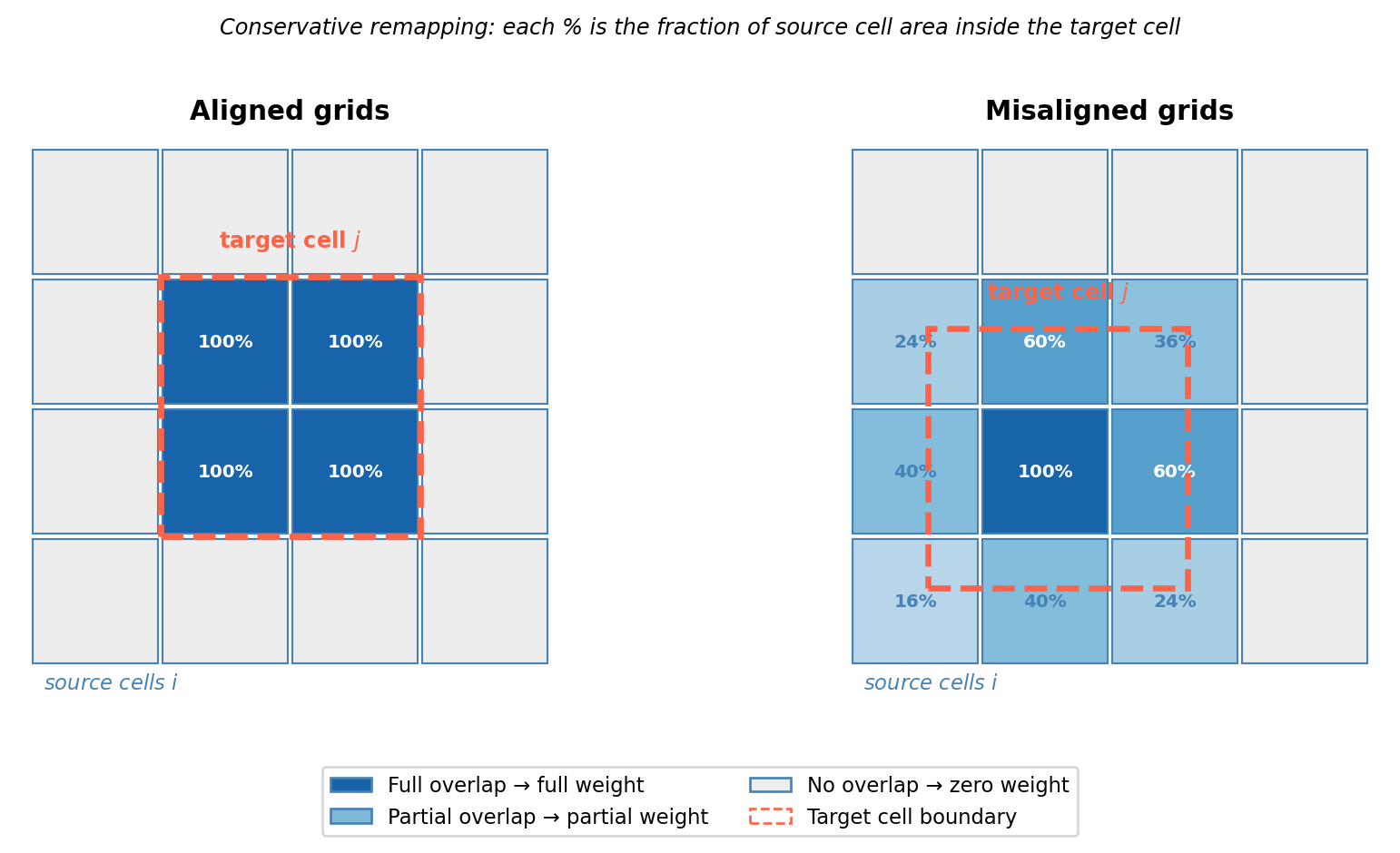
# Manual conservative (exact area-integral normalization, all in radians)
def block_conservative(ds_src, lats_tgt, lons_tgt, src_dlat=0.25, src_dlon=0.25):
    out = np.zeros((len(lats_tgt), len(lons_tgt)))
    tgt_dlat = abs(lats_tgt[1] - lats_tgt[0]) if len(lats_tgt) > 1 else 1.0
    tgt_dlon = abs(lons_tgt[1] - lons_tgt[0]) if len(lons_tgt) > 1 else 1.0
    for j, lt in enumerate(lats_tgt):
        for i, ln in enumerate(lons_tgt):
            mask_lat = (ds_src.lat >= lt - tgt_dlat/2) & (ds_src.lat < lt + tgt_dlat/2)
            mask_lon = (ds_src.lon >= ln - tgt_dlon/2) & (ds_src.lon < ln + tgt_dlon/2)
            sub = ds_src['precip'].isel(lat=mask_lat, lon=mask_lon)
            fine_lats = ds_src.lat.values[mask_lat]
            if sub.size > 0:
                # Fine cell areas in steradians: cos(lat) * dlat_rad * dlon_rad
                fine_areas = (np.cos(np.radians(fine_lats)) *
                              np.radians(src_dlat) * np.radians(src_dlon))[:, None]
                # Coarse cell area: exact integral of cos(lat) dlat dlon (all radians)
                coarse_area = ((np.sin(np.radians(lt + tgt_dlat/2))
                              - np.sin(np.radians(lt - tgt_dlat/2)))
                              * np.radians(tgt_dlon))
                out[j, i] = np.sum(sub.values * fine_areas) / coarse_area
    return out

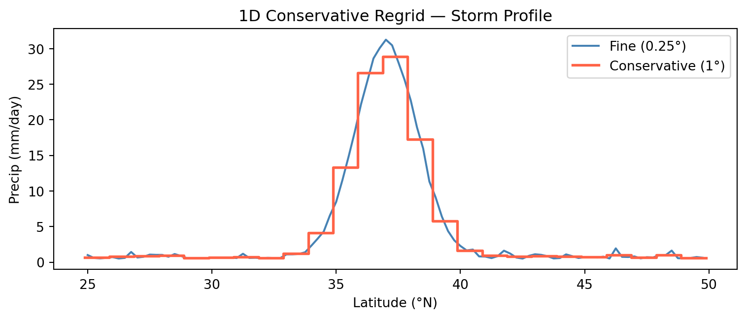
cons_vals = block_conservative(ds_fine, lats_c, lons_c)
ds_cons = xr.Dataset({'precip': (['lat','lon'], cons_vals, {'units':'mm/day'})},
                     coords={'lat': lats_c, 'lon': lons_c})

# Cell area proportional to cos(lat) * dlat * dlon — must include grid spacing or
# the fine grid (16× more cells) will give a 16× larger domain sum.
dlat_f, dlon_f = 0.25, 0.25
dlat_c, dlon_c = 1.0,  1.0
w_f = np.cos(np.radians(ds_fine.lat)) * dlat_f * dlon_f
w_c = np.cos(np.radians(ds_nn.lat))   * dlat_c * dlon_c
t_fine = float((ds_fine['precip'] * w_f).sum())
t_nn   = float((ds_nn['precip']   * w_c).sum())
t_bil  = float((ds_bil['precip']  * w_c).sum())
t_cons = float((ds_cons['precip'] * w_c).sum())

print(f"{'Method':<20} {'Total':>10} {'Error':>12} {'Peak':>10}")
print("-" * 56)
print(f"{'Fine (0.25°)':<20} {t_fine:>10.1f} {'—':>12} {float(ds_fine['precip'].max()):>10.2f}")
print(f"{'Nearest (1°)':<20} {t_nn:>10.1f} {(t_nn-t_fine)/t_fine*100:>10.2f}%  {float(ds_nn['precip'].max()):>10.2f}")
print(f"{'Bilinear (1°)':<20} {t_bil:>10.1f} {(t_bil-t_fine)/t_fine*100:>10.2f}%  {float(ds_bil['precip'].max()):>10.2f}")
print(f"{'Conservative (1°)':<20} {t_cons:>10.1f} {(t_cons-t_fine)/t_fine*100:>10.4f}%  {float(ds_cons['precip'].max()):>10.2f}")

Method                    Total        Error       Peak
--------------------------------------------------------
Fine (0.25°)             1674.7            —      21.72
Nearest (1°)             1682.3       0.45%       19.30
Bilinear (1°)            1682.3       0.45%       19.30
Conservative (1°)        1674.7     0.0013%       19.20

Why does this matter?

Nearest and bilinear both lose ~0.45% of the total precipitation budget every time you regrid. That sounds small — but applied globally over a year, or chained across multiple regridding steps in a pipeline, those errors compound.

Conservative remapping redistributes flux so the area-weighted integral is preserved to floating-point precision (~0.001%). For any budget-critical variable — precipitation, radiation, mass flux — this is the correct choice.

Rule of thumb:

Intensive variables (temperature, pressure, concentration): nearest or bilinear is fine
Extensive variables (precipitation, flux, mass): use conservative

Diagnostics: Always Validate Your Regridding

The Four Checks

After regridding, always run these four checks before using the output in analysis:

1. Domain mean

print(f"Source mean: {ds_source['precip'].mean().item():.3f}")
print(f"Target mean: {ds_target['precip'].mean().item():.3f}")
# For intensive vars: should be close
# For extensive vars: unweighted mean can change

2. Area-weighted integral (mass)

w = np.cos(np.radians(ds.lat))
mass_before = (ds_source['precip'] * w).sum().item()
mass_after  = (ds_target['precip'] * w).sum().item()
err = (mass_after - mass_before) / mass_before
print(f"Mass conservation error: {err*100:.4f}%")

3. Min / max values

print(f"Source: [{ds_source['precip'].min().item():.2f}, "
      f"{ds_source['precip'].max().item():.2f}]")
print(f"Target: [{ds_target['precip'].min().item():.2f}, "
      f"{ds_target['precip'].max().item():.2f}]")
# Bilinear can produce values outside original range
# Conservative stays within range

4. Difference map

diff = ds_target['precip'] - ds_source_coarsened['precip']
diff.plot(cmap='RdBu_r', center=0)
# Look for: systematic bias, edge artifacts, NaN propagation

A Complete Diagnostic Workflow

import numpy as np
import xarray as xr

rng = np.random.default_rng(42)
lats_f = np.arange(25, 50, 0.25)
lons_f = np.arange(-120, -70, 0.25)
LON, LAT = np.meshgrid(lons_f, lats_f)
T = 300 - 0.5*(LAT - 25) + 3*np.sin(np.radians(LON + 100))
T += rng.normal(0, 0.3, T.shape)
ds_src = xr.Dataset({'t2m': (['lat','lon'], T, {'units':'K'})},
                    coords={'lat': lats_f, 'lon': lons_f})

lats_c = np.arange(25.5, 50, 1.0)
lons_c = np.arange(-119.5, -70, 1.0)
ds_tgt = ds_src.interp(lat=lats_c, lon=lons_c)

def diagnose_regrid(ds_src, ds_tgt, varname):
    src = ds_src[varname]
    tgt = ds_tgt[varname]
    w_src = np.cos(np.radians(ds_src.lat))
    w_tgt = np.cos(np.radians(ds_tgt.lat))

    mass_src = float((src * w_src).sum())
    mass_tgt = float((tgt * w_tgt).sum())

    print(f"  Unweighted mean:   {float(src.mean()):.4f} → {float(tgt.mean()):.4f}")
    print(f"  Area-wtd integral: {mass_src:.2f} → {mass_tgt:.2f} "
          f"(err: {(mass_tgt-mass_src)/mass_src*100:.3f}%)")
    print(f"  Min/max:           [{float(src.min()):.2f}, {float(src.max()):.2f}] → "
          f"[{float(tgt.min()):.2f}, {float(tgt.max()):.2f}]")
    print(f"  NaN count in target: {int(tgt.isnull().sum())}")

print("Diagnostic: bilinear interpolation of temperature (0.25° → 1°)")
diagnose_regrid(ds_src, ds_tgt, 't2m')

Diagnostic: bilinear interpolation of temperature (0.25° → 1°)
  Unweighted mean:   294.0609 → 294.0104
  Area-wtd integral: 4642181.39 → 289606.42 (err: -93.761%)
  Min/max:           [286.04, 301.90] → [286.39, 301.30]
  NaN count in target: 0

What Acceptable Errors Look Like

No hard universal threshold — depends on context. Some guidelines:

Check	Intensive variable (T)	Extensive variable (precip)
Mean change	< 0.1 K acceptable	Any change is suspect
Mass error	< 1% acceptable	< 0.01% for conservative
Values outside range	Rare with bilinear	Should never happen with conservative
NaNs	Check edge handling	Check edge handling

Red flags to investigate:

NaNs at domain edges (boundary treatment issue)
Values outside the original range (extrapolation — check your coordinate bounds)
Large mean shift when coarsening temperature (suggests area-weighting issue)
Mass error > 0.1% with “conservative” method (bounds may be wrong)

Software Engineering Considerations

Design Patterns for Regridding Code

Good regridding code separates concerns:

Don’t do this:

# Recomputes weights every time — slow!
for year in range(1979, 2024):
    ds = xr.open_dataset(f'ERA5_{year}.nc')
    regridder = xe.Regridder(ds, target, 'bilinear')
    out = regridder(ds['t2m'])
    out.to_netcdf(f'out_{year}.nc')

Do this:

# Compute weights once, reuse
ds_template = xr.open_dataset('ERA5_1979.nc')
regridder = xe.Regridder(
    ds_template, target, 'bilinear'
)
regridder.to_netcdf('weights_bilinear.nc')

# All subsequent years: load weights
regridder = xe.Regridder(
    ds_template, target, 'bilinear',
    weights='weights_bilinear.nc'
)
for year in range(1979, 2024):
    ds = xr.open_dataset(f'ERA5_{year}.nc')
    regridder(ds['t2m']).to_netcdf(f'out_{year}.nc')

Document Your Grids

The single most common source of regridding bugs: not knowing what grid you’re on.

Always record in your dataset attributes:

import xarray as xr

ds_regridded = regridder(ds_source)

# Document what you did
ds_regridded.attrs.update({
    'regridding_method':  'bilinear',
    'source_grid':        '0.25deg ERA5',
    'target_grid':        '1.0deg CESM2',
    'regridding_tool':    'xESMF 0.8',
    'source_variable':    't2m',
    'regridded_by':       'your_name',
    'regridded_date':     '2026-02-20',
})

ds_regridded.to_netcdf('t2m_era5_on_cesm_grid.nc')

Tip

Future you will thank present you. Also: when you share data with collaborators, this metadata is the difference between a dataset they can use and one they have to ask you about.

Method Summary

Method	Smooth	Conservative	Typical Use	xarray / xESMF
Nearest neighbor	No	No	Masks, categorical	`.sel(method='nearest')`
Bilinear	Yes	No	Temperature, wind	`.interp()` / xESMF `'bilinear'`
Conservative	Moderate	Yes	Precipitation, fluxes	xESMF `'conservative'`

The decision tree:

Is the variable categorical or a mask?
  → Nearest neighbor

Is it an intensive variable (temperature, wind, pressure)?
  → Bilinear (for analysis) or nearest (for speed)

Is it an extensive variable (precip, energy flux)?
  → Conservative (always, for any scientific use)
  → Bilinear only if for visualization and you acknowledge the error

Practice

Lab: Conservation in Practice — Task 1

~25 minutes. Work in pairs. Submit by pushing your notebook to GitHub.

Task 1 (8 min) — Quantify the bilinear error

Create a precipitation field with a concentrated storm (Gaussian shape)
Regrid to 1° using bilinear interpolation
Run the full diagnostic (mean, mass, min/max, NaN count)
What fraction of mass is lost or gained?

import numpy as np, xarray as xr, matplotlib.pyplot as plt

# --- Setup (given) ---
rng   = np.random.default_rng(42)
lats_f = np.arange(25, 50, 0.25);  lons_f = np.arange(-120, -70, 0.25)
LON, LAT = np.meshgrid(lons_f, lats_f)
storm  = 30 * np.exp(-((LAT - 37)**2 / 3 + (LON + 100)**2 / 3))
precip = storm + 0.5 + rng.exponential(0.3, storm.shape)
ds_fine = xr.Dataset({'precip': (['lat','lon'], precip, {'units':'mm/day'})},
                      coords={'lat': lats_f, 'lon': lons_f})

# Bilinear regrid to 1°
lats_c = np.arange(25.5, 50, 1.0);  lons_c = np.arange(-119.5, -70, 1.0)
ds_bil = ds_fine.interp(lat=lats_c, lon=lons_c)

# --- Your turn ---
# Area weights:  cos(lat) * dlat_deg * dlon_deg
w_f = np.cos(np.radians(ds_fine.lat)) * 0.25 * 0.25   # shape (lat,)
w_c = ???

mass_fine = float((ds_fine['precip'] * w_f).sum())
mass_bil  = ???

print(f"Mass error: {(mass_bil - mass_fine) / mass_fine * 100:.3f}%")
# Also print: mean, min/max, NaN count for both grids

Lab: Conservation in Practice — Task 2

Task 2 (10 min) — Implement 1D conservative regridding

Using only numpy (no xESMF), fill in the ??? below:

def conservative_regrid_1d(f_src, src_edges, tgt_edges):
    """
    f_src:     source values  (n_src,)
    src_edges: source cell boundaries  (n_src + 1,)
    tgt_edges: target cell boundaries  (n_tgt + 1,)
    Returns:   target values  (n_tgt,)
    """
    n_tgt = len(tgt_edges) - 1
    out   = np.zeros(n_tgt)
    for i in range(n_tgt):
        t0, t1 = tgt_edges[i], tgt_edges[i + 1]
        # loop over source cells, accumulate weighted contributions
        for k in range(len(f_src)):
            s0, s1 = src_edges[k], src_edges[k + 1]
            overlap = ???          # length of [s0,s1] ∩ [t0,t1]
            out[i] += f_src[k] * overlap
        out[i] /= (t1 - t0)       # normalize by target cell width
    return out

# --- Test scaffold (given) ---
lon_idx   = np.argmin(np.abs(lons_f - (-100)))
f_src     = ds_fine['precip'].values[:, lon_idx]

src_dlat  = float(lats_f[1] - lats_f[0])
src_edges = np.append(lats_f - src_dlat / 2, lats_f[-1] + src_dlat / 2)
tgt_edges = np.arange(src_edges[0], src_edges[-1] + 0.001, 1.0)

f_tgt = conservative_regrid_1d(f_src, src_edges, tgt_edges)

# Mass check — should be 0.000000%
mass_before = np.sum(f_src * np.diff(src_edges))
mass_after  = np.sum(f_tgt * np.diff(tgt_edges))
print(f"1D mass error: {(mass_after - mass_before) / mass_before * 100:.6f}%")

# Plot: overlay fine (0.25°) and conservative (1°) profiles
tgt_ctrs = 0.5 * (tgt_edges[:-1] + tgt_edges[1:])
fig, ax  = plt.subplots(figsize=(8, 3.5))
ax.plot(???, ???, label='Fine (0.25°)')      # fine grid line
ax.step(???, ???, label='Conservative (1°)') # coarse step plot
ax.set_xlabel('Latitude (°N)');  ax.set_ylabel('Precip (mm/day)')
ax.legend();  plt.tight_layout();  plt.show()

Tip

Overlap hint: max(0, min(s1, t1) - max(s0, t0))

Key Takeaways

A grid is a geometric discretization. Lat/lon cells are not equal area — use area-weighted means.
Interpolation ≠ remapping. Interpolation estimates a value at a point. Conservative remapping redistributes a quantity while preserving the area integral.
The variable type determines the method. Intensive → bilinear fine. Extensive → conservative required.
Always diagnose your regridding. Mean, mass, min/max, NaN count. No exceptions.
Precompute and store weights. Regridding weights are expensive to compute and cheap to reuse.
Document everything. Source grid, target grid, method, tool, date — in the file attributes.

The core statement:

Regridding is not just interpolation for plotting. It changes the mathematical and physical properties of a dataset. The chosen method must be consistent with the physical meaning of the variable being remapped.

What’s Next

Week 10: Parallelization with Dask — now that you have tools to handle multiple grids, you need tools to handle multiple terabytes.

Recommended reading:

Jones (1999): “First- and Second-Order Conservative Remapping Schemes” — Monthly Weather Review
xESMF documentation: xesmf.readthedocs.io
Zender (2008): “Analysis of self-describing gridded geoscience data with netCDF Operators (NCO)”

Lab Solution

Lab Solution — Task 1: Quantify Bilinear Error

import numpy as np
import xarray as xr
import matplotlib.pyplot as plt

# Setup: Gaussian storm on 0.25-degree grid
rng = np.random.default_rng(0)
lats_f = np.arange(25, 50, 0.25)
lons_f = np.arange(-120, -70, 0.25)
LON, LAT = np.meshgrid(lons_f, lats_f)
storm = 30 * np.exp(-((LAT - 37)**2 / 3 + (LON + 100)**2 / 3))
precip = storm + 0.5 + rng.exponential(0.3, storm.shape)
ds_fine = xr.Dataset(
    {'precip': (['lat', 'lon'], precip, {'units': 'mm/day'})},
    coords={'lat': lats_f, 'lon': lons_f}
)

# Regrid to 1-degree using bilinear
lats_c = np.arange(25.5, 50, 1.0)
lons_c = np.arange(-119.5, -70, 1.0)
ds_bil = ds_fine.interp(lat=lats_c, lon=lons_c)

# Full diagnostics
w_f = np.cos(np.radians(ds_fine.lat)) * 0.25 * 0.25
w_c = np.cos(np.radians(ds_bil.lat))  * 1.0  * 1.0

mass_fine = float((ds_fine['precip'] * w_f).sum())
mass_bil  = float((ds_bil['precip']  * w_c).sum())

print("=== Diagnostic Report: Bilinear Regrid ===")
print(f"Source mean : {float(ds_fine['precip'].mean()):.4f} mm/day")
print(f"Target mean : {float(ds_bil['precip'].mean()):.4f} mm/day")
print(f"Mass before : {mass_fine:.2f}")
print(f"Mass after  : {mass_bil:.2f}")
print(f"Mass error  : {(mass_bil - mass_fine) / mass_fine * 100:.3f}%")
print(f"Source range: [{float(ds_fine['precip'].min()):.2f}, {float(ds_fine['precip'].max()):.2f}]")
print(f"Target range: [{float(ds_bil['precip'].min()):.2f}, {float(ds_bil['precip'].max()):.2f}]")
print(f"NaNs in target: {int(ds_bil['precip'].isnull().sum())}")

=== Diagnostic Report: Bilinear Regrid ===
Source mean : 1.0241 mm/day
Target mean : 1.0118 mm/day
Mass before : 1012.12
Mass after  : 997.29
Mass error  : -1.466%
Source range: [0.50, 31.26]
Target range: [0.50, 26.57]
NaNs in target: 0

Lab Solution — Task 2: Conservative Regrid 1D

def conservative_regrid_1d(f_src, src_edges, tgt_edges):
    """
    Conservative regridding in 1D.
    f_src:     values on source grid
    src_edges: source cell boundaries (len = len(f_src) + 1)
    tgt_edges: target cell boundaries (len = len(output) + 1)
    Returns: values on target grid, conserving the area-weighted integral
    """
    n_tgt = len(tgt_edges) - 1
    out = np.zeros(n_tgt)

    for i in range(n_tgt):
        t0, t1 = tgt_edges[i], tgt_edges[i + 1]
        tgt_width = t1 - t0
        weighted_sum = 0.0

        for k in range(len(f_src)):
            s0, s1 = src_edges[k], src_edges[k + 1]
            # overlap between source cell [s0, s1] and target cell [t0, t1]
            overlap = max(0.0, min(s1, t1) - max(s0, t0))
            if overlap > 0:
                weighted_sum += f_src[k] * overlap

        out[i] = weighted_sum / tgt_width  # normalize by target cell width

    return out

# Test: 1D latitude slice through storm center
lon_idx = np.argmin(np.abs(lons_f - (-100)))
f_src   = ds_fine['precip'].values[:, lon_idx]  # 100 values, centers at lats_f

# Build edges from cell centers: first/last edge = center +/- half-width
src_dlat  = float(lats_f[1] - lats_f[0])  # 0.25 deg
src_edges = np.append(lats_f - src_dlat / 2, lats_f[-1] + src_dlat / 2)
# [24.875, 25.125, ..., 49.875] — 101 edges for 100 cells

# Target: match outer domain exactly so no mass leaks at boundaries
tgt_edges = np.arange(src_edges[0], src_edges[-1] + 0.001, 1.0)
# [24.875, 25.875, ..., 49.875] — 26 edges, 25 cells
tgt_ctrs  = 0.5 * (tgt_edges[:-1] + tgt_edges[1:])

f_tgt = conservative_regrid_1d(f_src, src_edges, tgt_edges)

# Check conservation: integral (sum × cell width) before vs after
mass_before = np.sum(f_src * np.diff(src_edges))
mass_after  = np.sum(f_tgt * np.diff(tgt_edges))
print(f"1D mass before : {mass_before:.4f}")
print(f"1D mass after  : {mass_after:.4f}")
print(f"1D mass error  : {(mass_after - mass_before) / mass_before * 100:.6f}%")

# Plot comparison
fig, ax = plt.subplots(figsize=(8, 3.5))
ax.plot(lats_f, f_src, color='steelblue', linewidth=1.5, label='Fine (0.25°)')
ax.step(np.append(tgt_edges[:-1], tgt_edges[-1]),
        np.append(f_tgt, f_tgt[-1]),
        where='post', color='tomato', linewidth=2.0, label='Conservative (1°)')
ax.set_xlabel('Latitude (°N)')
ax.set_ylabel('Precip (mm/day)')
ax.set_title('1D Conservative Regrid — Storm Profile')
ax.legend()
plt.tight_layout()
plt.show()

1D mass before : 111.9600
1D mass after  : 111.9600
1D mass error  : 0.000000%