ATOC 4815/5815

Grids & Regridding I: Geometry and Interpolation — Week 9a

Will Chapman

CU Boulder ATOC

Spring 2026

Grids & Regridding I

Today’s Objectives

• Understand what a computational grid actually represents geometrically
• Recognize why lat/lon cells are not equal area
• Distinguish between interpolation and remapping
• Implement nearest-neighbor and bilinear interpolation with xarray
• Know when each method is appropriate
• Practice: regrid a real field with xarray and check what changed

The Problem We’re Solving

Last week: you worked with ERA5 at 0.25° resolution — one grid, no problem.

Reality of research:

ERA5 reanalysis:          0.25° × 0.25°  (~25 km)
CESM2 climate model:      ~1.0° × 1.0°   (~100 km)
IMERG precipitation:      0.1° × 0.1°    (~10 km)
GOES-16 satellite:        ~2 km
Your station obs:         a point

You need to combine these. How do you compare precipitation from IMERG (0.1°) to what a climate model (1°) produces? How do you subtract a reanalysis field from a satellite product?

You need to move data from one grid to another — that’s regridding.

Warning

Regridding is not just “making a plot look nicer.” It changes the mathematical and physical properties of your data. The method you choose matters.

What Is a Grid?

A Grid Is a Geometric Discretization

A grid is how we represent a continuous physical field using a finite set of numbers.

Continuous world:   T(lat, lon) — temperature at every point
Grid representation: T[i, j]   — temperature at grid cell centers

Structured grid (regular lat/lon)

• Regular spacing: Δλ, Δφ constant
• Each cell has a well-defined center and boundary
• Easy to index: T[lat_idx, lon_idx]
• ERA5, CESM, most reanalysis products

Unstructured grid

• Cells have variable shapes and sizes
• Used in some next-gen models (MPAS, ICON)
• Much harder to work with
• We focus on structured grids today

Key distinction:

• Grid cell center → where the value lives (what xarray coordinates represent)
• Grid cell boundary → edges of the cell (needed for conservative regridding)

The Geometry Problem: Cells Are Not Equal Area

This is the most important thing to internalize about lat/lon grids.

A 1° × 1° cell at the equator and a 1° × 1° cell near the pole cover very different physical areas.

The area of a lat/lon grid cell:

\[A(\phi) \approx R^2 \, \Delta\lambda \left( \sin\!\left(\phi + \tfrac{\Delta\phi}{2}\right) - \sin\!\left(\phi - \tfrac{\Delta\phi}{2}\right) \right)\]

where \(R\) = Earth’s radius, \(\phi\) = latitude, \(\Delta\lambda\), \(\Delta\phi\) = grid spacing in radians.

import numpy as np

R = 6371e3  # Earth radius in meters
dlat = np.radians(1.0)
dlon = np.radians(1.0)

lats = np.array([0, 30, 60, 80])
for phi in lats:
    phi_r = np.radians(phi)
    area = R**2 * dlon * (np.sin(phi_r + dlat/2) - np.sin(phi_r - dlat/2))
    area_km2 = area / 1e6
    print(f"  {phi:3d}°N:  {area_km2:,.0f} km²")

    0°N:  12,364 km²
   30°N:  10,708 km²
   60°N:  6,182 km²
   80°N:  2,147 km²

Cell Area — What This Means in Practice

A 1° cell at 80°N is ~6× smaller than a 1° cell at the equator.

Why does this matter?

If you naively average all grid cells equally, you are overweighting the poles.

import numpy as np

# Naive mean vs area-weighted mean
lats = np.arange(-89.5, 90.5, 1.0)
# Imagine a field = cos(lat): peak at equator, zero at poles
field = np.cos(np.radians(lats))

naive_mean = field.mean()

weights = np.cos(np.radians(lats))
weighted_mean = np.average(field, weights=weights)

print(f"Naive mean:         {naive_mean:.4f}")
print(f"Area-weighted mean: {weighted_mean:.4f}")

Naive mean:         0.6366
Area-weighted mean: 0.7854

The difference matters for global temperature trends, energy budgets, etc.

xarray makes area-weighting easy:

# Compute weights
weights = np.cos(np.radians(ds.lat))
weights.name = "weights"

# Weighted mean
ds['t2m'].weighted(weights).mean(dim=['lat','lon'])

You already know how to do this — we’re just being explicit about why it matters.

What Does Regridding Mean?

Two Different Operations, Same Word

People use “regridding” loosely. Be precise:

Interpolation

Estimate the value of a field at a new point based on surrounding values.

• Moving from coarse → fine: upsampling
• Moving from fine → coarse: downsampling
• No physical constraint — just geometry

Think: reading a thermometer between tick marks.

Conservative Remapping

Redistribute a quantity between grids such that the area-integrated total is preserved.

• Required for extensive quantities (precipitation, energy)
• Accounts for partial cell overlaps
• Physically meaningful

Think: redistributing flour between differently-sized measuring cups — the total amount doesn’t change.

Important

The correct choice depends on what the variable physically represents, not personal preference. We’ll return to this in Lecture 2.

Common Regridding Scenarios

Scenario	Direction	Typical Method
Climate model → obs comparison	Coarse → fine or fine → coarse	Bilinear or conservative
Combining two model outputs	Any	Match to common grid
Point obs → grid	Scatter → regular	Kriging, RBF, nearest
High-res satellite → model grid	Fine → coarse	Conservative
Visualization only	Any	Bilinear (fast, smooth)

The workflow is always: 1. Define your source grid and target grid 2. Choose a method appropriate to the variable 3. Apply the regridding 4. Validate — check that the result makes physical sense

Nearest-Neighbor Interpolation

Nearest Neighbor:

Definition: assign the value of the closest source grid point.

\[f_{\text{new}}(x, y) \rightarrow f(x_i, y_j) \quad \text{where } (x_i, y_j) = \arg\min \sqrt{(x-x_i)^2 + (y-y_j)^2}\]

Properties: - Discontinuous (blocky appearance) - Preserves original values exactly - Very fast - No smoothing — good or bad depending on context

Use when: - Land/sea masks - Categorical data (soil type, land cover class) - Index fields (basin ID, grid cell number) - When you cannot allow values that weren’t in the original data

You already know this:

# xarray: nearest neighbor selection
ds.sel(lat=40.0, lon=-105.0, method='nearest')

This is nearest-neighbor! You’ve been doing it since Week 5. Now you’re doing it for a whole grid.

# Regrid entire field to new lats/lons
new_lats = np.arange(20, 60, 2.0)
new_lons = np.arange(-130, -60, 2.0)

ds_nn = ds.sel(
    lat=new_lats,
    lon=new_lons,
    method='nearest'
)

Nearest Neighbor

import numpy as np
import xarray as xr
import matplotlib.pyplot as plt

# Build a synthetic fine-resolution temperature field (0.5° grid)
lats_fine = np.arange(25, 50, 0.5)
lons_fine = np.arange(-120, -70, 0.5)
LON, LAT = np.meshgrid(lons_fine, lats_fine)

# Realistic-ish temperature: warmer south, gradient east-west
T = 300 - 0.5 * (LAT - 25) + 3 * np.sin(np.radians(LON + 100))
T += np.random.default_rng(42).normal(0, 0.5, T.shape)

ds_fine = xr.Dataset(
    {'t2m': (['lat', 'lon'], T, {'units': 'K', 'long_name': '2m Temperature'})},
    coords={'lat': lats_fine, 'lon': lons_fine}
)

# Target: coarser 2° grid — nearest neighbor
lats_coarse = np.arange(26, 50, 2.0)
lons_coarse = np.arange(-119, -70, 2.0)

ds_nn = ds_fine.sel(lat=lats_coarse, lon=lons_coarse, method='nearest')
print(f"Fine grid:   {ds_fine['t2m'].shape}")
print(f"Coarse grid: {ds_nn['t2m'].shape}")
print(f"Fine mean:   {float(ds_fine['t2m'].mean()):.3f} K")
print(f"NN mean:     {float(ds_nn['t2m'].mean()):.3f} K")

Fine grid:   (50, 100)
Coarse grid: (12, 25)
Fine mean:   294.106 K
NN mean:     294.269 K

Notice the mean changes when you jump to a coarser grid — more on why that matters next lecture.

Bilinear Interpolation

Interpolate in Both Directions

Bilinear interpolation estimates the value at a new point by doing linear interpolation first in x, then in y (or equivalently, computing a weighted average of the four surrounding corner values).

For a target point \((x, y)\) inside a source cell with corners \((x_1, y_1), (x_2, y_2)\):

Define normalized coordinates: \[\alpha = \frac{x - x_1}{x_2 - x_1}, \quad \beta = \frac{y - y_1}{y_2 - y_1}, \quad \alpha, \beta \in [0, 1]\]

The four weights: \[w_1 = (1-\alpha)(1-\beta) \quad \text{(bottom-left)}\] \[w_2 = \alpha(1-\beta) \quad \text{(bottom-right)}\] \[w_3 = (1-\alpha)\beta \quad \text{(top-left)}\] \[w_4 = \alpha\beta \quad \text{(top-right)}\]

\[f(x,y) = w_1 f_1 + w_2 f_2 + w_3 f_3 + w_4 f_4\]

Geometric intuition:

A point right at corner 1 gets \(w_1 = 1\), all others zero.

A point at the center gets \(w_1 = w_2 = w_3 = w_4 = 0.25\) — an equal average of all four corners.

Points closer to a corner pull more weight from that corner.

Key property: the result is always a blend — values that didn’t exist in the original field can appear.

Bilinear — Properties and Trade-offs

Property	Nearest Neighbor	Bilinear
Continuity	Discontinuous	Continuous
Gradient preservation	Preserves sharp edges	Smooths gradients
Values outside original range	Never	Possible (extrapolation)
Conservation of integral	No	No
Speed	Very fast	Fast
Typical use	Masks, categorical	Temperature, wind, geopotential

Warning

The smoothing is a real problem. If you bilinearly interpolate daily precipitation from a fine grid to a coarse grid, you will spread the rain out and reduce peak intensity. For a temperature field, the smoothing is usually acceptable. Know your variable.

Discussion question: You have 3-hourly accumulated precipitation at 0.1° resolution. You want to compare it to a climate model at 1°. Should you use bilinear interpolation? What could go wrong?

Bilinear in xarray: .interp()

xarray’s .interp() method does bilinear interpolation natively.

import numpy as np
import xarray as xr

# Same fine-resolution dataset from before
lats_fine = np.arange(25, 50, 0.5)
lons_fine = np.arange(-120, -70, 0.5)
LON, LAT = np.meshgrid(lons_fine, lats_fine)
T = 300 - 0.5 * (LAT - 25) + 3 * np.sin(np.radians(LON + 100))
T += np.random.default_rng(42).normal(0, 0.5, T.shape)

ds_fine = xr.Dataset(
    {'t2m': (['lat', 'lon'], T, {'units': 'K'})},
    coords={'lat': lats_fine, 'lon': lons_fine}
)

# Target: 2° grid — bilinear interpolation
lats_coarse = np.arange(26, 50, 2.0)
lons_coarse = np.arange(-119, -70, 2.0)

ds_bilinear = ds_fine.interp(lat=lats_coarse, lon=lons_coarse)

print(f"Fine grid shape:     {ds_fine['t2m'].shape}")
print(f"Bilinear grid shape: {ds_bilinear['t2m'].shape}")
print(f"Fine mean:           {float(ds_fine['t2m'].mean()):.3f} K")
print(f"Bilinear mean:       {float(ds_bilinear['t2m'].mean()):.3f} K")

Fine grid shape:     (50, 100)
Bilinear grid shape: (12, 25)
Fine mean:           294.106 K
Bilinear mean:       294.269 K

.interp_like() — Match Another Dataset’s Grid

The most useful pattern in practice: you have two datasets on different grids and need to put them on the same one.

import numpy as np
import xarray as xr

# Dataset A: ERA5-like, 0.5° grid
lats_a = np.arange(25, 50, 0.5)
lons_a = np.arange(-120, -70, 0.5)
LON_a, LAT_a = np.meshgrid(lons_a, lats_a)
T_a = 300 - 0.5*(LAT_a - 25) + 3*np.sin(np.radians(LON_a + 100))
ds_era5 = xr.Dataset({'t2m': (['lat','lon'], T_a)},
                     coords={'lat': lats_a, 'lon': lons_a})

# Dataset B: Model output, 2° grid
lats_b = np.arange(26, 50, 2.0)
lons_b = np.arange(-118, -70, 2.0)
LON_b, LAT_b = np.meshgrid(lons_b, lats_b)
T_b = 298 - 0.4*(LAT_b - 25)
ds_model = xr.Dataset({'t2m': (['lat','lon'], T_b)},
                      coords={'lat': lats_b, 'lon': lons_b})

# Regrid ERA5 to model grid — one line
ds_era5_on_model_grid = ds_era5.interp_like(ds_model)

print(f"ERA5 grid:               {ds_era5['t2m'].shape}")
print(f"Model grid:              {ds_model['t2m'].shape}")
print(f"ERA5 regridded to model: {ds_era5_on_model_grid['t2m'].shape}")

# Now you can directly compare/subtract
bias = ds_model['t2m'] - ds_era5_on_model_grid['t2m']
print(f"Mean bias (model - ERA5): {float(bias.mean()):.2f} K")

ERA5 grid:               (50, 100)
Model grid:              (12, 24)
ERA5 regridded to model: (12, 24)
Mean bias (model - ERA5): -1.05 K

Comparing the Methods Visually

import numpy as np
import xarray as xr
import matplotlib.pyplot as plt

# Fine source field
lats_f = np.arange(25, 50, 0.5)
lons_f = np.arange(-120, -70, 0.5)
LON, LAT = np.meshgrid(lons_f, lats_f)
T = 300 - 0.5*(LAT - 25) + 3*np.sin(np.radians(LON+100))
T += np.random.default_rng(42).normal(0, 0.5, T.shape)
ds = xr.Dataset({'t2m': (['lat','lon'], T)}, coords={'lat': lats_f, 'lon': lons_f})

lats_c = np.arange(26, 50, 2.0)
lons_c = np.arange(-119, -70, 2.0)
ds_nn  = ds.sel(lat=lats_c, lon=lons_c, method='nearest')
ds_bil = ds.interp(lat=lats_c, lon=lons_c)

# Cross-section along a fixed latitude
lat_xs  = float(ds['t2m'].sel(lat=38.0, method='nearest').lat)
fine_xs = ds['t2m'].sel(lat=lat_xs, method='nearest')
nn_xs   = ds_nn['t2m'].sel(lat=lat_xs, method='nearest')
bil_xs  = ds_bil['t2m'].sel(lat=lat_xs, method='nearest')

from matplotlib.gridspec import GridSpec
fig = plt.figure(figsize=(13, 7))
gs  = GridSpec(2, 3, figure=fig, hspace=0.45, wspace=0.05,
               top=0.93, bottom=0.08, left=0.06, right=0.94)
ax_maps = [fig.add_subplot(gs[0, i]) for i in range(3)]
ax_xs   = fig.add_subplot(gs[1, :])

vmin, vmax = float(ds['t2m'].min()), float(ds['t2m'].max())
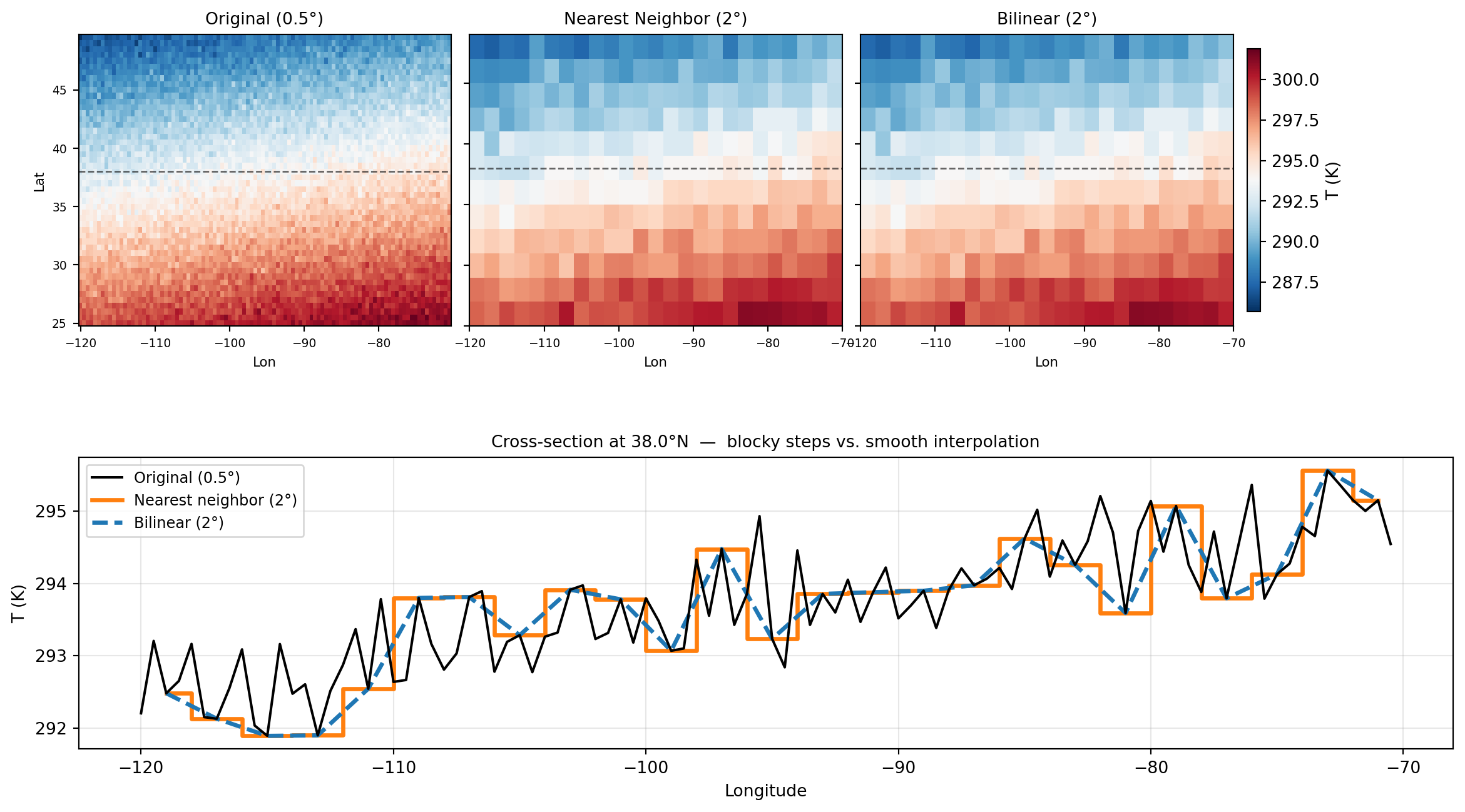
for ax, data, title in zip(ax_maps,
        [ds['t2m'], ds_nn['t2m'], ds_bil['t2m']],
        ['Original (0.5°)', 'Nearest Neighbor (2°)', 'Bilinear (2°)']):
    im = ax.pcolormesh(data.lon, data.lat, data.values,
                       vmin=vmin, vmax=vmax, cmap='RdBu_r')
    ax.set_title(title, fontsize=10)
    ax.set_xlabel('Lon', fontsize=8)
    ax.tick_params(labelsize=7)
    ax.axhline(lat_xs, color='k', lw=1, ls='--', alpha=0.6)
ax_maps[0].set_ylabel('Lat', fontsize=8)
for ax in ax_maps[1:]:
    ax.set_yticklabels([])
fig.colorbar(im, ax=ax_maps, shrink=0.9, pad=0.01, label='T (K)')

# Cross-section: the key comparison
ax_xs.plot(fine_xs.lon, fine_xs.values, 'k-',  lw=1.5, label='Original (0.5°)', zorder=3)
ax_xs.step(nn_xs.lon,   nn_xs.values,   where='mid',
           color='tab:orange', lw=2.5, label='Nearest neighbor (2°)')
ax_xs.plot(bil_xs.lon,  bil_xs.values,  '--',  lw=2.5,
           color='tab:blue', label='Bilinear (2°)', zorder=2)
ax_xs.set_xlabel('Longitude')
ax_xs.set_ylabel('T (K)')
ax_xs.set_title(f'Cross-section at {lat_xs:.1f}°N  —  blocky steps vs. smooth interpolation',
                fontsize=10)
ax_xs.legend(fontsize=9)
ax_xs.grid(alpha=0.3)

plt.savefig('/tmp/regrid_comparison.png', dpi=100, bbox_inches='tight')
plt.show()

Intensive vs. Extensive Variables

Physical Distinction Between Variables

Before you regrid anything, ask: what does this variable physically represent?

Intensive variables “does not scale with region size”

Double the area of a uniform-temperature region — the temperature does not double. It is still the same temperature.

• Temperature
• Wind speed / direction
• Pressure
• Specific humidity
• Geopotential height

→ Interpolation is fine. How you draw the grid cell does not change what temperature that location has.

Extensive variables “scales with region size”

Double the area — the total quantity doubles too. The value depends on how much area you are summing over.

• Daily precipitation accumulation
• Total evaporation
• Integrated radiative energy
• Cloud water path (column-integrated)

→ Interpolation is wrong. Bilinearly interpolating daily rainfall to a coarser grid changes the total amount of water in your domain.

The Conservation Equation

For extensive variables, regridding must satisfy:

\[\sum_i f_i \, A_i = \sum_j F_j \, A_j\]

where: - \(f_i\), \(A_i\) = values and areas on the source grid - \(F_j\), \(A_j\) = values and areas on the target grid

In plain English: the total amount (mass, energy, water) in the domain must be the same before and after regridding.

Bilinear interpolation does not guarantee this. Conservative remapping does.

We’ll build the math for conservative remapping next lecture.

Today’s takeaway question: You’re given daily IMERG precipitation at 0.1°. You want to compare it to CESM2 precipitation at 1°. Which method would you use and why?

Think about it — we’ll revisit at the start of next class.

Quick Reference: Method Selection

Variable	Type	Coarse → Fine	Fine → Coarse
Temperature	Intensive	Bilinear ✓	Bilinear ✓
Wind speed	Intensive	Bilinear ✓	Bilinear ✓
Land/sea mask	Categorical	Nearest neighbor ✓	Nearest neighbor ✓
Soil type	Categorical	Nearest neighbor ✓	Nearest neighbor ✓
Daily precip	Extensive	Bilinear (ok for viz)	Conservative
Radiative flux	Extensive	Bilinear (ok for viz)	Conservative

Note

“Fine → coarse” for extensive variables is where most mistakes happen in real research. When you aggregate 0.1° precipitation to 1°, you must use conservative remapping or your water budget will not close.

Practice

Lab: Regridding a Real Field

You have ~25 minutes. Work in pairs.

Setup: Create a synthetic dataset that mimics ERA5 temperature over the western US.

Task 1 (10 min) — Nearest Neighbor vs Bilinear:

1. Create a fine-grid (0.25°) temperature field with a realistic spatial pattern
2. Regrid it to 1° using nearest neighbor (.sel(method='nearest'))
3. Regrid it to 1° using bilinear (.interp())
4. Plot all three side by side
5. Print the mean of each. What do you notice?

Task 2 (10 min) — .interp_like():

1. Create a second dataset on a different grid (ERA5 0.5° + model 2°)
2. Use .interp_like() to put ERA5 on the model grid
3. Compute the difference field
4. Where is the difference largest? Why?

Task 3 (5 min) — Reflection:

For each variable below, write one sentence on which method you’d use and why:

• Daily precipitation totals
• 2m temperature
• Vegetation type (integer categories)
• Outgoing longwave radiation

Tip

Hint for Task 1: np.random.default_rng(42) for reproducibility. Use np.cos(np.radians(lat)) structure to make a realistic-looking temperature gradient.

What’s Next

Today: we built the geometric foundation and implemented nearest-neighbor + bilinear interpolation.

Next lecture (9b): We close the loop on extensive variables.

• The math of first-order conservative remapping
• How to implement it with xESMF (the production tool)
• Diagnosing whether your regridding preserved what it should
• Software engineering: precomputing weights, storing sparse matrices

Before next class: think about the precipitation question from the end of today. Bring your answer.

Key equation to remember:

\[A(\phi) \approx R^2 \, \Delta\lambda \left( \sin\!\left(\phi + \tfrac{\Delta\phi}{2}\right) - \sin\!\left(\phi - \tfrac{\Delta\phi}{2}\right) \right)\]

Grid cells are not equal area. Everything downstream of this fact matters.