ATOC 4815/5815

Tabular Data & Pandas Foundations - Week 7

Will Chapman

CU Boulder ATOC

Spring 2026

Tabular Data & Pandas

Today’s Objectives

• Understanding pandas: from arrays to tables
• Reading and parsing CSV files with dates
• Time series indexing and resampling
• Rolling windows and aggregations
• Creating publication-quality time series plots
• Recognizing and fixing common pandas errors
• Building analysis workflows you’ll use in research

Reminders

Due Friday at 9pm:

• Lab 4
• HW4

Office Hours:

Will: Tu / Th 11:15-12:15p

Aiden: M / W 4-5p

The Real Problem

Your Research Scenario

Imagine: You’re analyzing Boulder’s urban heat island effect

Your data:

• 10 ASOS weather stations around Boulder
• 1 year of hourly measurements (8,760 hours × 10 stations = 87,600 rows!)
• Multiple variables: temperature, humidity, wind speed, pressure, precipitation

Each station CSV looks like:

Date and Time,Station,Temp_C,RH_pct,Wind_kt,Pressure_hPa,Precip_mm
2024-01-01 00:00,KBDU,2.1,65,8,1013.2,0.0
2024-01-01 01:00,KBDU,1.8,68,7,1013.5,0.0
2024-01-01 02:00,KBDU,1.2,71,6,1013.8,0.2
...

Questions you need to answer:

1. What’s the average daily temperature at each station?
2. Which station is warmest? When?
3. How does precipitation accumulate over the month?
4. Are there heat waves (3+ consecutive days > 30°C)?

Why NumPy Arrays Fall Short

Try solving this with NumPy arrays…

Problem 1: Multiple data types

# NumPy arrays must be uniform type
temps = np.array([2.1, 1.8, 1.2])  # ✅ Works
times = np.array(['2024-01-01 00:00', '2024-01-01 01:00'])  # ✅ Works
mixed = np.array(['KBDU', 2.1, 65])  # ❌ Everything becomes strings!

Problem 2: No column names

# How do you remember which column is which?
data = np.array([
    [2.1, 65, 8, 1013.2, 0.0],  # Station 1, hour 1
    [1.8, 68, 7, 1013.5, 0.0],  # Station 1, hour 2
])
# Is column 1 temp or humidity? Have to check your notes!

Problem 3: Time-based operations are painful

# "Give me hourly data resampled to daily" requires:
# - Manual grouping by date
# - Index math to find boundaries
# - Custom aggregation loops
# This is 20+ lines of error-prone code!

What Pandas Gives Us

Pandas solves all these problems:

1. Mixed data types in columns:

df['Station']      # Strings
df['Temp_C']       # Floats
df['Date and Time'] # Timestamps
# Each column can be different!

2. Named columns:

df['Temp_C']  # Clear what you're accessing
df['RH_pct']  # No guessing column indices

3. Time-aware operations:

# Resample hourly to daily in one line:
daily = df.resample('1D').mean()

# Rolling 24-hour average:
df['temp_24h'] = df['Temp_C'].rolling('24h').mean()

Bottom line: For tabular data with time series, Pandas is the right tool. NumPy is for uniform numeric arrays and math.

Why Pandas?

Pandas Scientific Story

Created by Wes McKinney (late 2000s) to handle panel data for quantitative finance

• Goal: bring R/Excel/SQL-style table tools into Python

Built on top of NumPy, adding:

• Labeled rows/columns (DataFrame, Series)
• Easy handling of missing values
• Powerful time-series tools (date indexes, resampling, rolling windows)

Became the standard tabular data library in scientific Python:

• Most data tutorials start with import pandas as pd
• Common front-end for reading/writing CSV, Excel, SQL, NetCDF/Parquet, etc.
• Feeds directly into NumPy, Matplotlib, and higher-level tools (xarray, geopandas, statsmodels)

For this course, think of pandas as:

“Excel + SQL + NumPy, but in code” — a single place to clean data, compute statistics, and drive time-series visualizations.

Mental Model: NumPy vs Pandas

Think of it this way:

NumPy:        "Calculator for arrays of numbers"
              ✅ Fast math, vectorized operations
              ❌ No column names, no mixed types, weak time handling

Pandas:       "Spreadsheet + database in Python"
              ✅ Named columns, mixed types, time series tools
              ✅ Built on NumPy (uses arrays internally)
              ❌ Slightly slower (but worth it for convenience)

Use NumPy when:

• Doing heavy numerical computation (matrix ops, FFT, stats)
• All data is numeric and uniform

Use Pandas when:

• Working with tables (CSV, Excel, SQL)
• Have mixed data types (strings, dates, numbers)
• Need time-based operations (resampling, rolling windows)
• Want readable code with named columns

Check Your Understanding

Which tool should you use for each task?

1. Computing the FFT of 10,000 temperature measurements

Answer: NumPy (uniform numeric array, pure math operation)

2. Loading a CSV with station names, timestamps, temps, and wind speeds

Answer: Pandas (mixed types, labeled columns, time data)

3. Calculating daily mean temperature from hourly data

Answer: Pandas (time-based resampling with .resample('1D').mean())

4. Multiplying two 1000×1000 matrices

Answer: NumPy (pure numeric computation with np.dot() or @)

Pandas Fundamentals

Series: One Column

A Series is a 1-D labeled array (like one column of a spreadsheet)

import pandas as pd
import numpy as np

# Create a Series
temps = pd.Series([15.2, 18.7, 22.1, 19.8],
                  index=['Mon', 'Tue', 'Wed', 'Thu'])
print(temps)

Mon    15.2
Tue    18.7
Wed    22.1
Thu    19.8
dtype: float64

Key features:

• .index → row labels (Mon, Tue, Wed, Thu)
• .values → underlying NumPy array
• Access by label: temps['Mon'] → 15.2
• Access by position: temps[0] → 15.2

DataFrame: Multiple Series

A DataFrame is a 2-D table (like a whole spreadsheet)

# Create a DataFrame
data = pd.DataFrame({
    'temp_c': [15.2, 18.7, 22.1, 19.8],
    'pressure_hpa': [1010, 1012, 1008, 1011]
}, index=['Mon', 'Tue', 'Wed', 'Thu'])
print(data)

     temp_c  pressure_hpa
Mon    15.2          1010
Tue    18.7          1012
Wed    22.1          1008
Thu    19.8          1011

Key features:

• .columns → column names (temp_c, pressure_hpa)
• .index → row labels (Mon, Tue, Wed, Thu)
• Each column is a Series
• Access column: data['temp_c'] → Series
• Access row: data.loc['Mon'] → Series

Common Error: Accessing Columns

Predict the output:

import pandas as pd

df = pd.DataFrame({
    'temp_c': [15.2, 18.7, 22.1],
    'station': ['KBDU', 'KDEN', 'KBJC']
})

print(df.temp_c)  # Does this work?

0    15.2
1    18.7
2    22.1
Name: temp_c, dtype: float64

✅ It works! But there’s a catch…

The Problem:

# ✅ Good: Always use bracket notation
df['temp_c']

# ⚠️ Risky: Dot notation fails if column name has spaces or conflicts
df.temp c      # SyntaxError!
df.max         # Gets the method, not a column named 'max'!

Best practice: Always use df['column_name'] for columns

Common Error: KeyError

Predict the output:

df = pd.DataFrame({
    'temp_c': [15.2, 18.7, 22.1],
    'station': ['KBDU', 'KDEN', 'KBJC']
})

print(df['temperature'])  # What happens?

KeyError: 'temperature'

Explanation: Column ‘temperature’ doesn’t exist (it’s ‘temp_c’)

The Fix:

# Check available columns first
print(df.columns)  # Index(['temp_c', 'station'], dtype='object')

# Or use .get() with a default
value = df.get('temperature', default=None)  # Returns None instead of error

Common causes:

• Typo in column name
• Wrong capitalization (‘Temp_C’ vs ‘temp_c’)
• Column was renamed or not read from CSV

Try It Yourself 💻

With your neighbor (3 min): Create a DataFrame with Boulder weather

weather = pd.DataFrame({
    'date': ['2024-01-01', '2024-01-02', '2024-01-03'],
    'temp_c': [2.1, 3.5, 1.2],
    'precip_mm': [0.0, 2.5, 0.5]
})

# Tasks:
# 1. Print the DataFrame
# 2. Extract just the temp_c column
# 3. What's the maximum precipitation?
# 4. Try accessing a column that doesn't exist—what error do you get?

Answers:

# 1.
print(weather)

# 2.
temps = weather['temp_c']

# 3.
max_precip = weather['precip_mm'].max()  # 2.5

# 4.
weather['humidity']  # KeyError: 'humidity'

Reading Data

Reading CSVs: The Wrong Way

What happens if you just read the CSV naively?

# Sample CSV as a string (simulating a file)
import io
csv_data = """Date and Time,Station,Temp_C
2024-01-01 00:00,KBDU,2.1
2024-01-01 01:00,KBDU,1.8
2024-01-01 02:00,KBDU,1.2"""

df_wrong = pd.read_csv(io.StringIO(csv_data))
print(df_wrong)
print(f"\nData type of 'Date and Time': {df_wrong['Date and Time'].dtype}")

      Date and Time Station  Temp_C
0  2024-01-01 00:00    KBDU     2.1
1  2024-01-01 01:00    KBDU     1.8
2  2024-01-01 02:00    KBDU     1.2

Data type of 'Date and Time': object

Problem: ‘Date and Time’ is stored as a string (object), not a timestamp!

Why it matters:

• Can’t do time-based operations (resampling, rolling windows)
• Can’t filter by date easily
• Can’t extract month, day, hour

Reading CSVs: The Right Way

Use parse_dates to convert string → datetime:

csv_data = """Date and Time,Station,Temp_C
2024-01-01 00:00,KBDU,2.1
2024-01-01 01:00,KBDU,1.8
2024-01-01 02:00,KBDU,1.2"""

df_right = pd.read_csv(io.StringIO(csv_data), parse_dates=['Date and Time'])
print(df_right)
print(f"\nData type of 'Date and Time': {df_right['Date and Time'].dtype}")

        Date and Time Station  Temp_C
0 2024-01-01 00:00:00    KBDU     2.1
1 2024-01-01 01:00:00    KBDU     1.8
2 2024-01-01 02:00:00    KBDU     1.2

Data type of 'Date and Time': datetime64[ns]

Now it’s a datetime64 type!

What you can do now:

# Extract components
print(f"Hour of first row: {df_right['Date and Time'][0].hour}")

# Filter by date
after_midnight = df_right[df_right['Date and Time'] >= '2024-01-01 01:00']
print(f"\nRows after midnight: {len(after_midnight)}")

Hour of first row: 0

Rows after midnight: 2

Common Error: Forgetting parse_dates

Predict the output:

# CSV read WITHOUT parse_dates
df = pd.read_csv('weather.csv')  # Forgot parse_dates!

# Try to resample to daily
daily = df.resample('1D').mean()

TypeError: Only valid with DatetimeIndex, TimedeltaIndex or PeriodIndex,
but got an instance of 'RangeIndex'

Explanation: Can’t resample without a time index!

The Fix:

# Method 1: Parse on read
df = pd.read_csv('weather.csv', parse_dates=['Date and Time'])
df = df.set_index('Date and Time')
daily = df.resample('1D').mean()  # ✅ Works!

# Method 2: Convert after reading
df = pd.read_csv('weather.csv')
df['Date and Time'] = pd.to_datetime(df['Date and Time'])
df = df.set_index('Date and Time')

Setting a Time Index

For time series analysis, make the timestamp the index

Why?

• Enables .resample(), .rolling(), time-based slicing
• Aligns operations by time automatically
• Makes plots use time on x-axis by default

# Create sample data
dates = pd.date_range('2024-01-01', periods=5, freq='h')
df = pd.DataFrame({
    'temp_c': [15.2, 16.1, 17.3, 18.2, 17.5],
    'pressure_hpa': [1010, 1011, 1009, 1008, 1010]
}, index=dates)

print(df)
print(f"\nIndex type: {type(df.index)}")

                     temp_c  pressure_hpa
2024-01-01 00:00:00    15.2          1010
2024-01-01 01:00:00    16.1          1011
2024-01-01 02:00:00    17.3          1009
2024-01-01 03:00:00    18.2          1008
2024-01-01 04:00:00    17.5          1010

Index type: <class 'pandas.core.indexes.datetimes.DatetimeIndex'>

Now time-based operations work:

# Time-based slicing
print("\n2-hour window:")
print(df['2024-01-01 02:00':'2024-01-01 04:00'])

2-hour window:
                     temp_c  pressure_hpa
2024-01-01 02:00:00    17.3          1009
2024-01-01 03:00:00    18.2          1008
2024-01-01 04:00:00    17.5          1010

Setting Index: Two Methods

Method 1: Set index after reading

df = pd.read_csv('weather.csv', parse_dates=['Date and Time'])
df = df.set_index('Date and Time')

Method 2: Set index during read (more efficient)

df = pd.read_csv('weather.csv',
                 parse_dates=['Date and Time'],
                 index_col='Date and Time')

Method 2 is better:

• One step instead of two
• Slightly faster (one less copy)
• Less code to maintain

Check Your Understanding

What’s wrong with this code?

df = pd.read_csv('boulder_weather.csv')
daily_mean = df.resample('1D').mean()

Two problems:

1. ❌ No parse_dates — dates are strings, not datetimes
2. ❌ No time index set — can’t resample without DatetimeIndex

The fix:

df = pd.read_csv('boulder_weather.csv',
                 parse_dates=['Date and Time'],
                 index_col='Date and Time')
daily_mean = df.resample('1D').mean()  # ✅ Now it works!

Resampling & Aggregation

What is Resampling?

Resampling: Change the frequency of your time series

Visual example:

Hourly data (24 points per day):
├─ 00:00 → 15.2°C
├─ 01:00 → 16.1°C
├─ 02:00 → 17.3°C
├─ 03:00 → 18.2°C
   ...

Resample to daily (1 point per day):
└─ 2024-01-01 → 16.7°C (mean of all 24 hours)

Common patterns:

• Downsampling: High → Low frequency (hourly → daily)
• Aggregation: How to combine values (mean, sum, max, min, etc.)

Resampling Syntax

# Create 15-minute data
dates = pd.date_range('2024-01-01', periods=96, freq='15min')
df = pd.DataFrame({
    'temp_c': 15 + 5 * np.sin(np.arange(96) * 2 * np.pi / 96) + np.random.randn(96) * 0.5,
    'precip_mm': np.random.exponential(0.1, 96)
}, index=dates)

print("Original (15-min):")
print(df.head())

# Resample to hourly
hourly = df.resample('1h').mean()

print("\nResampled (hourly):")
print(hourly.head())

Original (15-min):
                        temp_c  precip_mm
2024-01-01 00:00:00  13.914531   0.180880
2024-01-01 00:15:00  15.385386   0.068789
2024-01-01 00:30:00  16.241221   0.116100
2024-01-01 00:45:00  16.737492   0.000390
2024-01-01 01:00:00  16.066743   0.129261

Resampled (hourly):
                        temp_c  precip_mm
2024-01-01 00:00:00  15.569658   0.091540
2024-01-01 01:00:00  16.637765   0.331263
2024-01-01 02:00:00  17.616016   0.028853
2024-01-01 03:00:00  19.055411   0.042044
2024-01-01 04:00:00  19.497183   0.035190

Aggregation Rules: When to Use What?

Different variables need different aggregation methods:

Variable	Aggregation	Why?
Temperature	mean()	Average temp over period makes sense
Precipitation	sum()	Want total accumulated precip
Wind speed	mean() or max()	Mean for typical, max for gusts
Pressure	mean()	Average pressure over period
Station ID	first()	Metadata—just keep one

Example:

# Different rules for different columns
hourly = df.resample('1h').agg({
    'temp_c': 'mean',      # Average temperature
    'precip_mm': 'sum'     # Total precipitation
})

print(hourly.head(3))

                        temp_c  precip_mm
2024-01-01 00:00:00  15.569658   0.366160
2024-01-01 01:00:00  16.637765   1.325053
2024-01-01 02:00:00  17.616016   0.115412

Common Error: Wrong Aggregation

Predict the problem:

# 24 hours of precipitation data
precip = pd.Series([0.5, 0.2, 0.0, 0.8, ...], index=hourly_times)

# Resample to daily
daily_precip = precip.resample('1D').mean()  # ❌ WRONG!

The Problem: Using mean() for precipitation!

• You don’t want the “average hourly precip”
• You want “total daily precip”

The Fix:

daily_precip = precip.resample('1D').sum()  # ✅ Correct!

Example:

Hourly:  [0.5, 0.2, 0.0, 0.8] mm
Daily (wrong): mean = 0.375 mm  ← What does this even mean?
Daily (right): sum = 1.5 mm      ← Total precip for the day

Try It Yourself 💻

With your neighbor (5 min): Practice resampling

# Create hourly temperature data
dates = pd.date_range('2024-01-01', periods=168, freq='h')  # 1 week
temps = pd.Series(
    15 + 8 * np.sin(np.arange(168) * 2 * np.pi / 24) + np.random.randn(168),
    index=dates
)

# Tasks:
# 1. Resample to daily mean temperature
# 2. Find the warmest day
# 3. Resample to 6-hour max temperature
# 4. What happens if you resample but forget to call .mean() or .sum()?

Answers:

# 1. Daily mean
daily = temps.resample('1D').mean()

# 2. Warmest day
warmest = daily.idxmax()  # Returns the date
print(f"Warmest day: {warmest} at {daily.max():.1f}°C")

# 3. 6-hour max
six_hour_max = temps.resample('6h').max()

# 4. Forget aggregation
resampled = temps.resample('1D')  # Just returns a Resampler object, not data!
print(resampled)  # DatetimeIndexResampler [freq=<Day>, ...]

Multiple Aggregations

You can compute multiple statistics at once:

# Create sample data
dates = pd.date_range('2024-01-01', periods=168, freq='h')
df = pd.DataFrame({
    'temp_c': 15 + 8 * np.sin(np.arange(168) * 2 * np.pi / 24) + np.random.randn(168) * 2,
    'precip_mm': np.random.exponential(0.3, 168)
}, index=dates)

# Daily aggregation with different rules
daily = df.resample('1D').agg({
    'temp_c': ['mean', 'min', 'max'],
    'precip_mm': 'sum'
})

print(daily)

               temp_c                      precip_mm
                 mean       min        max       sum
2024-01-01  14.580122  4.843042  23.222845  7.183108
2024-01-02  15.474521  5.838430  23.170576  7.648080
2024-01-03  15.055395  4.956987  22.427721  4.967984
2024-01-04  15.274361  5.513813  26.523146  4.792476
2024-01-05  15.073889  3.441440  23.863967  3.620983
2024-01-06  14.697729  5.576067  25.173492  6.044943
2024-01-07  14.789997  5.416497  25.023515  7.493903

Accessing multi-level columns:

# Access specific aggregation
daily_mean_temp = daily['temp_c']['mean']
daily_precip = daily['precip_mm']['sum']

print(f"\nFirst day mean temp: {daily_mean_temp.iloc[0]:.1f}°C")
print(f"First day total precip: {daily_precip.iloc[0]:.2f} mm")

First day mean temp: 14.6°C
First day total precip: 7.18 mm

Resampling Frequency Codes

Common frequency strings:

Code	Meaning	Example
'1h'	Hourly	Every hour
'3h'	Every 3 hours	00:00, 03:00, 06:00, …
'1D'	Daily	Once per day
'1W'	Weekly	Once per week
'1MS'	Monthly (start)	First day of each month
'1ME'	Monthly (end)	Last day of each month
'1QS'	Quarterly (start)	Jan 1, Apr 1, Jul 1, Oct 1
'1YS'	Yearly (start)	Jan 1 each year

You can combine numbers and codes:

df.resample('6h').mean()    # Every 6 hours
df.resample('15min').sum()  # Every 15 minutes
df.resample('2W').max()     # Every 2 weeks

Check Your Understanding

For each scenario, which aggregation should you use?

1. Converting hourly temperature to daily

Answer: mean() — average temperature for the day

2. Converting 5-minute rainfall to hourly

Answer: sum() — total rainfall accumulated per hour

3. Converting hourly wind speed to daily

Answer: Could use mean() for typical wind, or max() for peak gusts

4. Converting hourly pressure to 6-hour

Answer: mean() — average pressure over 6-hour period

Rolling Windows

What is a Rolling Window?

Rolling window: Compute statistics over a moving time window

Visual example:

Data:     [10, 12, 15, 18, 20, 22, 21, 19, 16, 14]
           ↓   ↓   ↓
Window:   [10, 12, 15]  → mean = 12.3
               ↓   ↓   ↓
Window:       [12, 15, 18]  → mean = 15.0
                   ↓   ↓   ↓
Window:           [15, 18, 20]  → mean = 17.7
                       ...

Result: A smoothed version of the original data

Rolling Window Syntax

# Create hourly temperature data
dates = pd.date_range('2024-01-01', periods=168, freq='h')
temps = pd.Series(
    15 + 8 * np.sin(np.arange(168) * 2 * np.pi / 24) + np.random.randn(168) * 2,
    index=dates
)

# Rolling means with different windows
temps_3h = temps.rolling('3h').mean()
temps_12h = temps.rolling('12h').mean()
temps_24h = temps.rolling('24h').mean()

print("Original vs Rolling means:")
df_compare = pd.DataFrame({
    'original': temps,
    'rolling_3h': temps_3h,
    'rolling_12h': temps_12h,
    'rolling_24h': temps_24h
})
print(df_compare.head(26))

Original vs Rolling means:
                      original  rolling_3h  rolling_12h  rolling_24h
2024-01-01 00:00:00  13.430573   13.430573    13.430573    13.430573
2024-01-01 01:00:00  18.303263   15.866918    15.866918    15.866918
2024-01-01 02:00:00  19.605840   17.113225    17.113225    17.113225
2024-01-01 03:00:00  20.449199   19.452767    17.947219    17.947219
2024-01-01 04:00:00  23.016047   21.023695    18.960984    18.960984
2024-01-01 05:00:00  26.571005   23.345417    20.229321    20.229321
2024-01-01 06:00:00  26.049987   25.212346    21.060845    21.060845
2024-01-01 07:00:00  24.199208   25.606733    21.453140    21.453140
2024-01-01 08:00:00  19.750425   23.333206    21.263950    21.263950
2024-01-01 09:00:00  17.846706   20.598780    20.922225    20.922225
2024-01-01 10:00:00  18.147368   18.581500    20.669966    20.669966
2024-01-01 11:00:00  15.824490   17.272855    20.266176    20.266176
2024-01-01 12:00:00  13.334491   15.768783    20.258169    19.732969
2024-01-01 13:00:00  16.064426   15.074469    20.071599    19.470930
2024-01-01 14:00:00   7.465181   12.288032    19.059878    18.670547
2024-01-01 15:00:00   7.511461   10.347022    17.981733    17.973104
2024-01-01 16:00:00  11.774505    8.917049    17.044938    17.608481
2024-01-01 17:00:00   9.713914    9.666627    15.640180    17.169894
2024-01-01 18:00:00   5.642003    9.043474    13.939515    16.563163
2024-01-01 19:00:00   5.765302    7.040407    12.403356    16.023270
2024-01-01 20:00:00   8.039077    6.482127    11.427410    15.643070
2024-01-01 21:00:00   9.685630    7.830003    10.747321    15.372277
2024-01-01 22:00:00  11.484880    9.736529    10.192113    15.203260
2024-01-01 23:00:00  15.650739   12.273749    10.177634    15.221905
2024-01-02 00:00:00  12.222016   13.119211    10.084928    15.171548
2024-01-02 01:00:00  19.104951   15.659235    10.338305    15.204952

Rolling Window Visualization

import matplotlib.pyplot as plt

# Plot raw data and rolling means
plt.figure(figsize=(9, 4))
plt.plot(temps.index, temps, alpha=0.3, label='Raw (hourly)', linewidth=1)
plt.plot(temps.index, temps_3h, label='3-hour rolling mean', linewidth=1.5)
plt.plot(temps.index, temps_12h, label='12-hour rolling mean', linewidth=1.5)
plt.plot(temps.index, temps_24h, label='24-hour rolling mean', linewidth=2)
plt.xlabel('Date')
plt.ylabel('Temperature (°C)')
plt.title('Temperature with Rolling Means')
plt.legend()
plt.grid(True, alpha=0.3)
plt.tight_layout()
plt.show()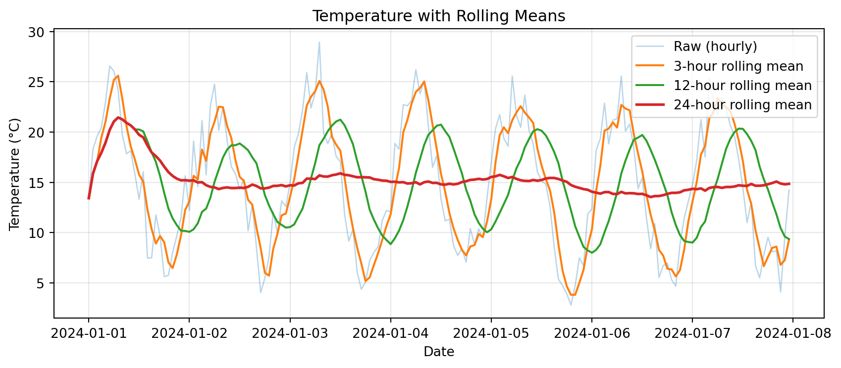

Notice: Longer windows → smoother curves, but more lag

Rolling vs Resampling: What’s the Difference?

Resampling: Change frequency (hourly → daily)

• Reduces number of points
• Each point represents a whole period

Rolling: Smooth data over a moving window

• Same number of points (except edge NaNs)
• Each point is an average of nearby points

Example:

# Original: 168 hourly points
print(f"Original: {len(temps)} points")

# Resampling to daily: reduces to 7 points
daily = temps.resample('1D').mean()
print(f"Resampled daily: {len(daily)} points")

# Rolling 24-hour: still 168 points (but first 23 are NaN)
rolling_24h = temps.rolling('24h').mean()
print(f"Rolling 24h: {len(rolling_24h)} points (includes NaN at start)")

Original: 168 points
Resampled daily: 7 points
Rolling 24h: 168 points (includes NaN at start)

Common Error: Rolling on Wrong Data Type

Predict the output:

df = pd.DataFrame({
    'station': ['KBDU', 'KBDU', 'KBDU', 'KBDU'],
    'temp_c': [15.2, 16.1, 17.3, 18.2]
})

# Try rolling mean on station names
rolling = df['station'].rolling(3).mean()

TypeError: unsupported operand type(s) for /: 'str' and 'int'

Explanation: Can’t compute mean of strings!

The Fix:

# ✅ Rolling on numeric data
rolling = df['temp_c'].rolling(3).mean()

# ✅ Or select numeric columns only
rolling = df.select_dtypes(include=[np.number]).rolling(3).mean()

Rolling Statistics Beyond Mean

Rolling windows aren’t just for means:

# Create temperature data
dates = pd.date_range('2024-01-01', periods=168, freq='h')
temps = pd.Series(
    15 + 8 * np.sin(np.arange(168) * 2 * np.pi / 24) + np.random.randn(168) * 2,
    index=dates
)

# Different rolling statistics
rolling_mean = temps.rolling('24h').mean()
rolling_std = temps.rolling('24h').std()
rolling_min = temps.rolling('24h').min()
rolling_max = temps.rolling('24h').max()

print("Rolling 24-hour statistics:")
print(pd.DataFrame({
    'mean': rolling_mean,
    'std': rolling_std,
    'min': rolling_min,
    'max': rolling_max
}).describe())

Rolling 24-hour statistics:
             mean         std         min         max
count  168.000000  167.000000  168.000000  168.000000
mean    15.299953    5.925789    5.873312   24.900191
std      1.472864    0.928368    3.026600    1.472259
min     13.933582    1.642869    4.156660   15.550696
25%     14.502460    5.861707    4.385326   23.837734
50%     14.939480    6.188527    4.718021   25.242903
75%     15.213846    6.385266    6.102354   25.667605
max     21.015377    6.880182   15.550696   26.631479

Use Case: Temperature Variability

Rolling standard deviation shows how variable conditions are:

# Create data with changing variability
dates = pd.date_range('2024-01-01', periods=168, freq='h')
# Add more noise in second half
noise = np.concatenate([
    np.random.randn(84) * 1,    # Low variability
    np.random.randn(84) * 4     # High variability
])
temps = pd.Series(
    15 + 8 * np.sin(np.arange(168) * 2 * np.pi / 24) + noise,
    index=dates
)

rolling_mean = temps.rolling('12h').mean()
rolling_std = temps.rolling('12h').std()

# Plot
fig, (ax1, ax2) = plt.subplots(2, 1, figsize=(9, 5), sharex=True)

ax1.plot(temps.index, temps, alpha=0.4, label='Hourly temp')
ax1.plot(temps.index, rolling_mean, linewidth=2, label='12-h mean')
ax1.set_ylabel('Temperature (°C)')
ax1.set_title('Temperature and Variability')
ax1.legend()
ax1.grid(True, alpha=0.3)

ax2.plot(temps.index, rolling_std, color='red', linewidth=2)
ax2.set_xlabel('Date')
ax2.set_ylabel('Rolling Std Dev (°C)')
ax2.set_title('12-hour Rolling Variability')
ax2.grid(True, alpha=0.3)

plt.tight_layout()
plt.show()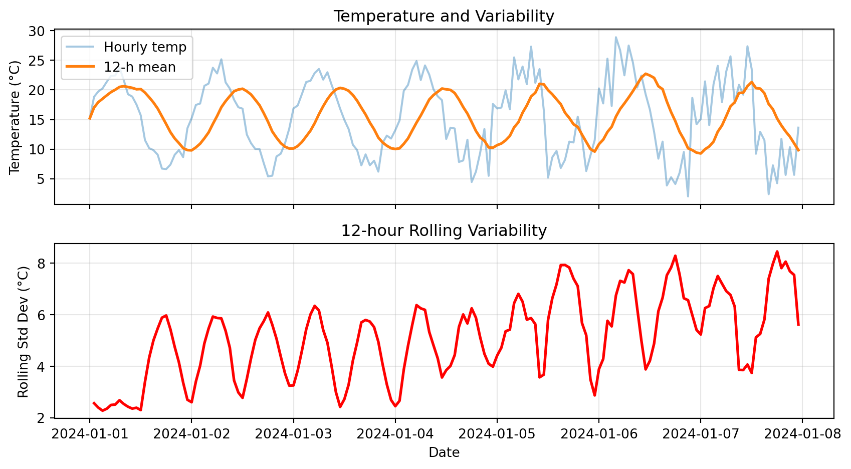

Notice: High rolling std in second half → more variable conditions

Try It Yourself 💻

With your neighbor (5 min): Explore rolling windows

# Create 1 week of hourly wind speed data
dates = pd.date_range('2024-01-01', periods=168, freq='h')
wind_kt = pd.Series(
    10 + 5 * np.abs(np.sin(np.arange(168) * 2 * np.pi / 24)) + np.random.randn(168) * 2,
    index=dates
)

# Tasks:
# 1. Compute 6-hour rolling mean wind speed
# 2. Find the time period with highest 6-hour average wind
# 3. Compute 12-hour rolling max (for peak gusts)
# 4. What's the difference between .rolling(6) and .rolling('6h')?

Answers:

# 1. 6-hour rolling mean
rolling_mean_6h = wind_kt.rolling('6h').mean()

# 2. Highest 6-hour average
max_time = rolling_mean_6h.idxmax()
max_wind = rolling_mean_6h.max()
print(f"Highest 6-h avg wind: {max_wind:.1f} kt at {max_time}")

# 3. 12-hour rolling max
rolling_max_12h = wind_kt.rolling('12h').max()

# 4. Difference:
# .rolling(6) → 6 data points (may not be 6 hours if data is irregular)
# .rolling('6h') → 6 hours of data (time-aware, handles gaps correctly)

Anomalies & Cumulative Sums

Computing Anomalies

Anomaly: Deviation from a baseline (climatology, daily mean, etc.)

Why anomalies matter:

• Identify unusual events
• Remove seasonal cycle
• Compare different stations or years

Example: Hourly temperature anomalies from daily mean

# Create hourly data for a week
dates = pd.date_range('2024-01-01', periods=168, freq='h')
temps = pd.Series(
    15 + 8 * np.sin(np.arange(168) * 2 * np.pi / 24) + np.random.randn(168) * 2,
    index=dates
)
df = pd.DataFrame({'temp_c': temps})

# Method: use groupby to compute daily mean, then subtract
df['date'] = df.index.date
df['daily_mean'] = df.groupby('date')['temp_c'].transform('mean')
df['anomaly'] = df['temp_c'] - df['daily_mean']

print(df[['temp_c', 'daily_mean', 'anomaly']].head(10))

                        temp_c  daily_mean   anomaly
2024-01-01 00:00:00  12.763851   15.179458 -2.415607
2024-01-01 01:00:00  20.588715   15.179458  5.409257
2024-01-01 02:00:00  17.395535   15.179458  2.216077
2024-01-01 03:00:00  18.002869   15.179458  2.823411
2024-01-01 04:00:00  20.187423   15.179458  5.007965
2024-01-01 05:00:00  19.883463   15.179458  4.704005
2024-01-01 06:00:00  24.675903   15.179458  9.496445
2024-01-01 07:00:00  21.795617   15.179458  6.616159
2024-01-01 08:00:00  19.511111   15.179458  4.331653
2024-01-01 09:00:00  22.947661   15.179458  7.768203

Visualizing Anomalies

# Plot raw data and anomalies
fig, (ax1, ax2) = plt.subplots(2, 1, figsize=(9, 5), sharex=True)

# Top: Raw temperature
ax1.plot(df.index, df['temp_c'], label='Hourly temp', alpha=0.7)
ax1.plot(df.index, df['daily_mean'], label='Daily mean', linewidth=2, color='red')
ax1.set_ylabel('Temperature (°C)')
ax1.set_title('Raw Temperature and Daily Mean')
ax1.legend()
ax1.grid(True, alpha=0.3)

# Bottom: Anomalies
ax2.plot(df.index, df['anomaly'], color='purple', alpha=0.7)
ax2.axhline(y=0, color='black', linestyle='--', linewidth=1)
ax2.set_xlabel('Date')
ax2.set_ylabel('Anomaly (°C)')
ax2.set_title('Hourly Anomalies from Daily Mean')
ax2.grid(True, alpha=0.3)

plt.tight_layout()
plt.show()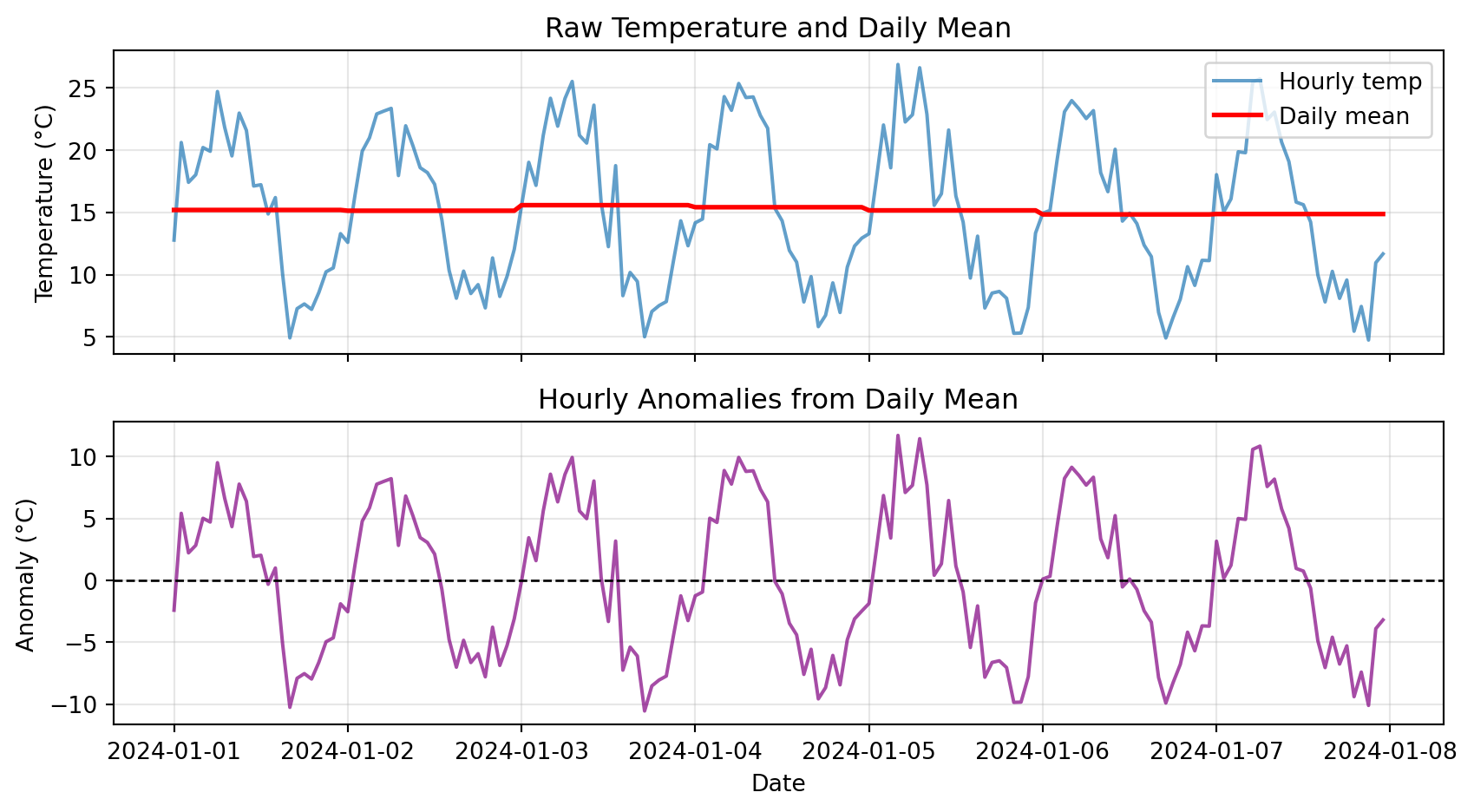

Notice: Anomalies oscillate around zero, showing deviations from typical pattern

Cumulative Sums

Cumulative sum: Running total over time

Use cases:

• Precipitation: Total accumulated rainfall
• Energy: Cumulative power consumption
• Degree-days: Accumulated heat or cold

# Create precipitation data
dates = pd.date_range('2024-01-01', periods=168, freq='h')
precip = pd.Series(np.random.exponential(0.3, 168), index=dates)

# Compute cumulative sum
cumulative = precip.cumsum()

print("Hourly and cumulative precipitation:")
print(pd.DataFrame({
    'hourly_mm': precip,
    'cumulative_mm': cumulative
}).head(10))

Hourly and cumulative precipitation:
                     hourly_mm  cumulative_mm
2024-01-01 00:00:00   0.603929       0.603929
2024-01-01 01:00:00   0.249990       0.853919
2024-01-01 02:00:00   0.020977       0.874896
2024-01-01 03:00:00   0.158153       1.033049
2024-01-01 04:00:00   0.746480       1.779529
2024-01-01 05:00:00   0.155099       1.934628
2024-01-01 06:00:00   0.388143       2.322771
2024-01-01 07:00:00   0.009408       2.332179
2024-01-01 08:00:00   0.799203       3.131382
2024-01-01 09:00:00   0.249677       3.381059

Cumulative Precipitation Visualization

# Plot hourly and cumulative
fig, (ax1, ax2) = plt.subplots(2, 1, figsize=(9, 5), sharex=True)

# Top: Hourly bars
ax1.bar(precip.index, precip, width=0.04, alpha=0.6, color='steelblue')
ax1.set_ylabel('Hourly Precip (mm)')
ax1.set_title('Hourly Precipitation')
ax1.grid(True, alpha=0.3)

# Bottom: Cumulative line
ax2.plot(cumulative.index, cumulative, linewidth=2, color='darkblue')
ax2.set_xlabel('Date')
ax2.set_ylabel('Cumulative Precip (mm)')
ax2.set_title('Cumulative Precipitation')
ax2.grid(True, alpha=0.3)

plt.tight_layout()
plt.show()

print(f"\nTotal precipitation over week: {cumulative.iloc[-1]:.2f} mm")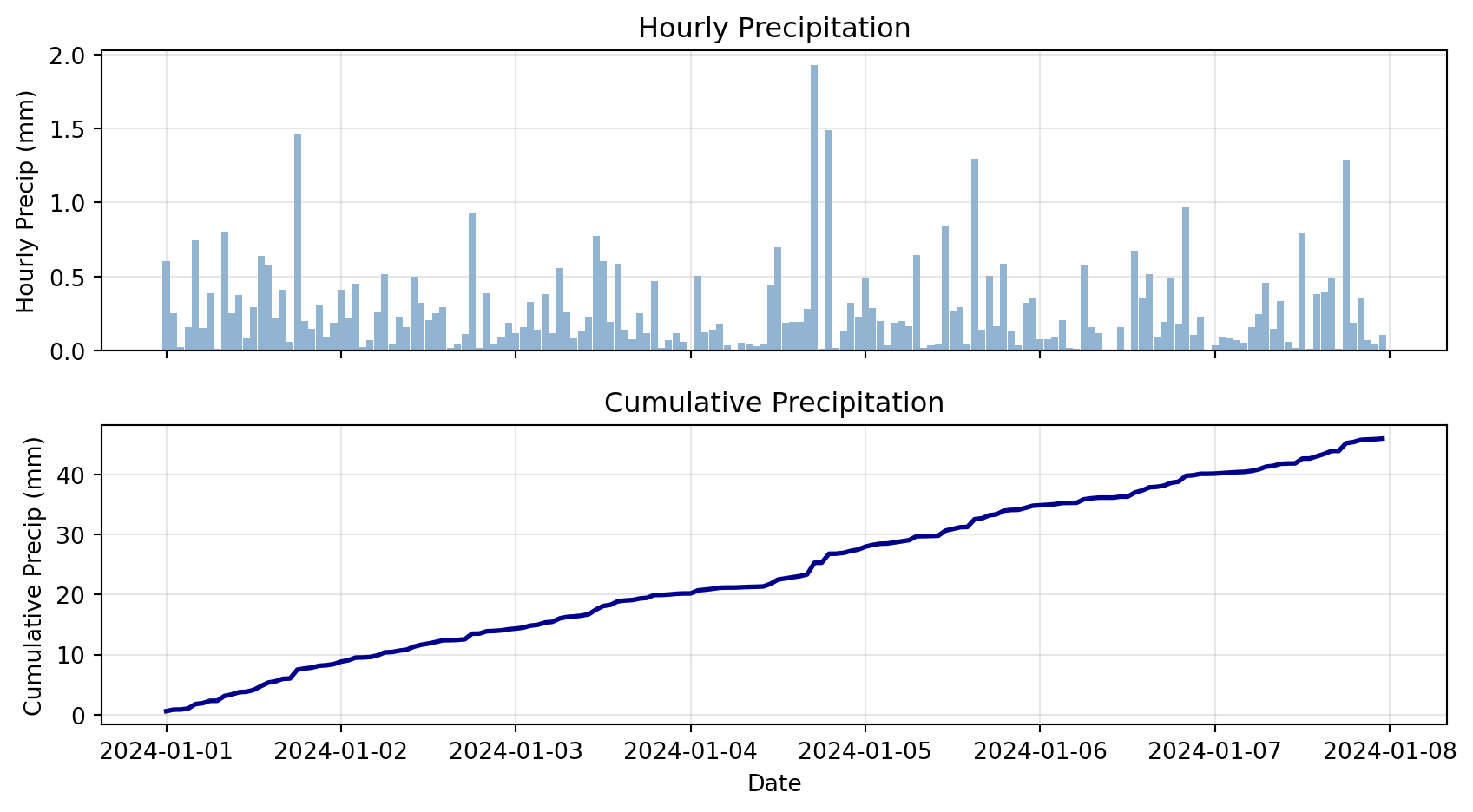

Total precipitation over week: 45.97 mm

Check Your Understanding

Match each technique to its use case:

Techniques:

1. Rolling mean
2. Resampling
3. Anomaly
4. Cumulative sum

Use cases:

A. “How much total rainfall since Jan 1?”

B. “What’s the smoothed temperature trend?”

C. “Convert hourly data to daily averages”

D. “How much warmer than normal was today?”

Answers:

1-B (Rolling mean → smoothing)

2-C (Resampling → change frequency)

3-D (Anomaly → deviation from baseline)

4-A (Cumulative sum → total accumulated)

Plotting Time Series

Pandas Native Plotting

Pandas DataFrames have built-in .plot() method:

# Create sample data
dates = pd.date_range('2024-01-01', periods=168, freq='h')
df_plot = pd.DataFrame({
    'temp_c': 15 + 8 * np.sin(np.arange(168) * 2 * np.pi / 24) + np.random.randn(168) * 2,
}, index=dates)
df_plot['rolling_24h'] = df_plot['temp_c'].rolling('24h').mean()

# Simple plot
df_plot.plot(
    figsize=(9, 4),
    title='Temperature Time Series',
    ylabel='Temperature (°C)',
    grid=True,
    alpha=0.7
)
plt.tight_layout()
plt.show()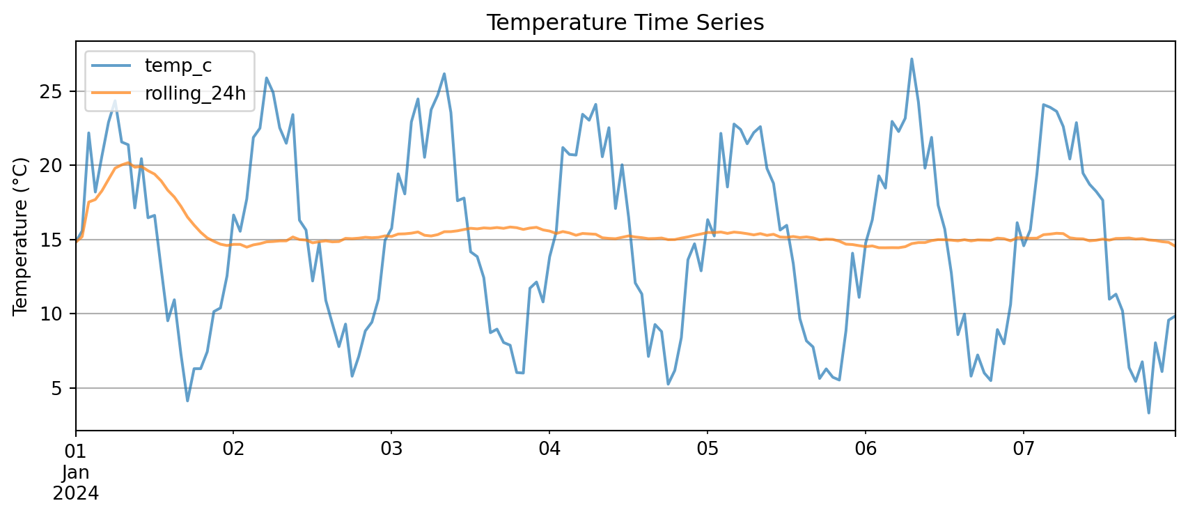

Key advantage: .plot() automatically uses the index as x-axis

Multi-Panel Time Series

For complex analysis, use matplotlib subplots:

# Create comprehensive dataset
dates = pd.date_range('2024-01-01', periods=168, freq='h')
weather = pd.DataFrame({
    'temp_c': 15 + 8 * np.sin(np.arange(168) * 2 * np.pi / 24) + np.random.randn(168) * 2,
    'rh_pct': 60 + 20 * np.sin(np.arange(168) * 2 * np.pi / 24 + np.pi/4) + np.random.randn(168) * 5,
    'precip_mm': np.random.exponential(0.3, 168)
}, index=dates)

# Add derived quantities
weather['temp_rolling_24h'] = weather['temp_c'].rolling('24h').mean()
weather['cumulative_precip'] = weather['precip_mm'].cumsum()

# Create multi-panel plot
fig, (ax1, ax2, ax3) = plt.subplots(3, 1, figsize=(9, 7), sharex=True)

# Panel 1: Temperature
ax1.plot(weather.index, weather['temp_c'], alpha=0.4, label='Hourly Temp')
ax1.plot(weather.index, weather['temp_rolling_24h'], linewidth=2, label='24-h Rolling Mean')
ax1.set_ylabel('Temperature (°C)')
ax1.set_title('Weather Time Series Analysis')
ax1.legend(loc='best')
ax1.grid(True, alpha=0.3)

# Panel 2: Relative Humidity
ax2.plot(weather.index, weather['rh_pct'], color='green', alpha=0.7)
ax2.set_ylabel('Relative Humidity (%)')
ax2.grid(True, alpha=0.3)

# Panel 3: Precipitation (dual y-axes)
ax3.bar(weather.index, weather['precip_mm'], width=0.04, alpha=0.6, label='Hourly Precip')
ax3_cum = ax3.twinx()
ax3_cum.plot(weather.index, weather['cumulative_precip'], color='steelblue',
             linewidth=2, label='Cumulative')
ax3.set_xlabel('Date')
ax3.set_ylabel('Hourly Precip (mm)')
ax3_cum.set_ylabel('Cumulative (mm)')
ax3.legend(loc='upper left')
ax3_cum.legend(loc='upper right')
ax3.grid(True, alpha=0.3)

plt.tight_layout()
plt.show()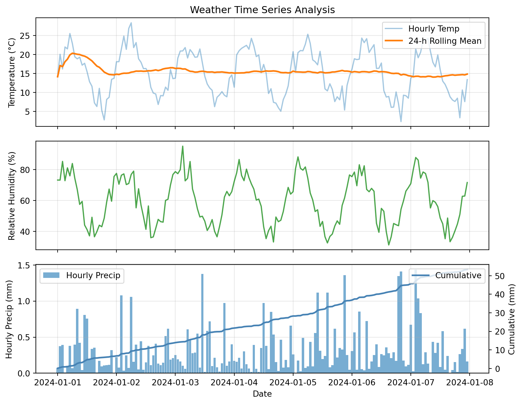

This plot combines:

• Raw and smoothed time series (top)
• Secondary variables (middle)
• Dual y-axes for different scales (bottom)

Advanced Topics

Boolean Filtering with Time Index

With a time index, boolean masks work just like NumPy:

# Create precipitation data
dates = pd.date_range('2024-01-01', periods=168, freq='h')
precip_df = pd.DataFrame({
    'precip_mm': np.random.exponential(0.3, 168)
}, index=dates)

# Boolean mask: rainy hours (> 0.5 mm)
rainy_hours = precip_df['precip_mm'] > 0.5

# Count and extract
print(f"Number of rainy hours: {rainy_hours.sum()}")
print(f"\nRainiest hours:")
print(precip_df[rainy_hours].nlargest(5, 'precip_mm'))

Number of rainy hours: 33

Rainiest hours:
                     precip_mm
2024-01-05 21:00:00   1.632770
2024-01-07 22:00:00   1.533483
2024-01-04 20:00:00   1.386506
2024-01-07 15:00:00   1.168597
2024-01-07 21:00:00   1.115051

Combine conditions:

# Hot and dry conditions
hot_dry = (weather['temp_c'] > 30) & (weather['rh_pct'] < 20)

# Cold or very wet
cold_wet = (weather['temp_c'] < 0) | (weather['precip_mm'] > 5)

Helper Functions for Reusable Analysis

Instead of copy-pasting analysis code, wrap it in functions:

def summarize_period(df, freq='1D', temp_col='temp_c', precip_col='precip_mm'):
    """
    Resample time series to specified frequency.

    Parameters
    ----------
    df : pd.DataFrame
        Input dataframe with time index
    freq : str
        Resample frequency ('1h', '1D', '1W', etc.)
    temp_col : str
        Name of temperature column
    precip_col : str
        Name of precipitation column

    Returns
    -------
    pd.DataFrame
        Resampled data with mean temp and total precip
    """
    # Check that required columns exist
    if temp_col not in df.columns:
        raise ValueError(f"Column '{temp_col}' not found in DataFrame")
    if precip_col not in df.columns:
        raise ValueError(f"Column '{precip_col}' not found in DataFrame")

    # Resample with appropriate aggregations
    summary = df.resample(freq).agg({
        temp_col: ['mean', 'min', 'max'],
        precip_col: 'sum'
    })
    return summary

# Test the function
daily_summary = summarize_period(weather, freq='1D', temp_col='temp_c', precip_col='precip_mm')
print(daily_summary)

               temp_c                      precip_mm
                 mean       min        max       sum
2024-01-01  14.640377  2.773482  25.515810  6.539472
2024-01-02  16.502022  6.835782  28.336740  7.123112
2024-01-03  15.185221  6.254272  21.817022  7.943578
2024-01-04  15.223711  5.062103  24.245138  6.394275
2024-01-05  15.540580  5.376075  25.325979  8.560953
2024-01-06  14.414805  2.328391  24.315043  8.516529
2024-01-07  14.836209  3.334557  24.255768  8.263232

Benefits:

• Reusable across projects
• Easy to test and debug
• One place to update logic
• Handles errors gracefully

Common Error: Missing Values in Rolling

Predict the output:

temps = pd.Series([15, 18, np.nan, 22, 19], index=pd.date_range('2024-01-01', periods=5, freq='h'))

rolling = temps.rolling(3).mean()
print(rolling)

2024-01-01 00:00:00      NaN
2024-01-01 01:00:00      NaN
2024-01-01 02:00:00      NaN  ← Missing value propagates!
2024-01-01 03:00:00      NaN
2024-01-01 04:00:00     20.5

By default, NaN in window → NaN result

The Fix:

# Skip NaN values in rolling calculation
rolling = temps.rolling(3, min_periods=1).mean()
# OR
rolling = temps.rolling(3).mean(skipna=True)  # Default behavior

When to Use Each Tool

Decision guide:

Goal	Tool	Example
Change frequency	.resample()	Hourly → daily
Smooth noisy data	.rolling().mean()	Remove high-freq noise
Total accumulated	.cumsum()	Total rainfall since Jan 1
Deviation from normal	Anomaly (subtract baseline)	Temp - climatology
Find extreme periods	Boolean mask + filter	Hours where temp > 35°C
Compare different aggregations	.resample().agg({...})	Daily mean temp, total precip

Bonus Challenge 💻

Design a ‘heatwave detector’ that flags multi-day warm spells

Task: Create a function find_heatwaves(df, temp_col='temp_c', threshold=30, min_duration=72) that returns a list of (start_time, end_time, peak_temp) for every period where temperature stays above threshold for at least min_duration consecutive hours.

Hints:

1. Create boolean Series: df[temp_col] > threshold
2. Use .diff() or .ne() with .cumsum() to label contiguous blocks
3. Aggregate each block: compute duration and peak temperature
4. Filter for blocks meeting min_duration requirement
5. Return list of (start, end, peak) tuples

Example solution:

def find_heatwaves(df, temp_col='temp_c', threshold=30, min_duration=72):
    """Detect heatwaves in temperature time series.

    Parameters
    ----------
    df : pd.DataFrame
        Input dataframe with time index
    temp_col : str
        Name of temperature column
    threshold : float
        Temperature threshold (°C)
    min_duration : int
        Minimum duration in hours

    Returns
    -------
    list of tuples
        Each tuple: (start_time, end_time, peak_temp)
    """
    # Create boolean mask
    is_hot = df[temp_col] > threshold

    # Label contiguous blocks (changes create new block IDs)
    blocks = (is_hot != is_hot.shift()).cumsum()

    # Filter for hot blocks only
    hot_blocks = blocks[is_hot]

    # Compute duration and peak for each block
    heatwaves = []
    for block_id in hot_blocks.unique():
        block_mask = blocks == block_id
        block_data = df[block_mask]
        duration = len(block_data)

        if duration >= min_duration:
            start = block_data.index[0]
            end = block_data.index[-1]
            peak = block_data[temp_col].max()
            heatwaves.append((start, end, peak))

    return heatwaves

# Test it
test_dates = pd.date_range('2024-06-01', periods=240, freq='h')
test_temps = 20 + 10 * np.sin(np.arange(240) * 2 * np.pi / 24) + np.random.randn(240) * 2
test_temps[50:130] += 10  # Add a heatwave
test_df = pd.DataFrame({'temp_c': test_temps}, index=test_dates)

heatwaves = find_heatwaves(test_df, threshold=28, min_duration=48)
print(f"Found {len(heatwaves)} heatwave(s):")
for start, end, peak in heatwaves:
    duration = (end - start).total_seconds() / 3600
    print(f"  {start} to {end} ({duration:.0f} hours), peak: {peak:.1f}°C")

Summary & Resources

Key Concepts Review

1. Pandas gives us labeled tables for mixed data types

• Series (1D) and DataFrames (2D)
• Named columns and time indexes

2. Reading CSVs: use parse_dates and index_col

• Converts strings to datetime objects
• Sets time index for time-aware operations

3. Resampling: change frequency

• Downsampling: high → low frequency
• Choose aggregation method: mean, sum, max, etc.

4. Rolling windows: smooth data

• Moving averages over time
• Same number of points (except NaNs at edges)

5. Anomalies: deviations from baseline

• Subtract climatology or daily mean
• Identifies unusual events

6. Cumulative sums: running totals

• Total accumulated precipitation, energy, etc.

Common Errors to Avoid

1. Forgetting parse_dates

# ❌ Dates are strings
df = pd.read_csv('data.csv')

# ✅ Dates are datetime objects
df = pd.read_csv('data.csv', parse_dates=['Date and Time'])

2. No time index before resampling

# ❌ Can't resample without time index
df.resample('1D').mean()

# ✅ Set time index first
df = df.set_index('Date and Time')
df.resample('1D').mean()

3. Wrong aggregation method

# ❌ Mean precipitation doesn't make sense
precip_daily = df['precip_mm'].resample('1D').mean()

# ✅ Sum precipitation for totals
precip_daily = df['precip_mm'].resample('1D').sum()

4. Using .rolling(n) instead of .rolling('nh')

# ⚠️ 24 data points (may not be 24 hours if gaps exist)
df.rolling(24).mean()

# ✅ 24 hours of data (time-aware)
df.rolling('24h').mean()

Assignment Checklist

Due Friday at 9pm:

• Lab 4
• HW4

HW4 will cover:

• Loading CSV data with parse_dates and index_col
• Setting time index for resampling
• Resampling to different frequencies (hourly → daily)
• Computing anomalies from climatology
• Rolling window statistics for smoothing
• Creating multi-panel time series plots
• Writing helper functions for reusable analysis

Start early! Time series analysis has many moving parts.

Resources and Support

Available to you:

• Lab notebooks with step-by-step examples
• Office hours (bring your data questions!)
• Discussion channels
• Pandas docs: pandas.pydata.org
• Stack Overflow for specific error messages

Learning tip: Pandas takes practice. Start simple:

1. Load data → print it
2. Set index → check it worked
3. Try one operation → verify output
4. Build up complexity gradually

Remember: The time index is your friend—most pandas time series power comes from having a proper DatetimeIndex!

Questions?

Contact

Prof. Will Chapman

📧 wchapman@colorado.edu

🌐 willychap.github.io

🏢 ATOC Building, CU Boulder

Office Hours: Tu/Th 11:15-12:15p

See you next week!