Time-averaged temperature (one value per grid point):
Shape: (20, 20)
<xarray.DataArray 't2m' (lat: 20, lon: 20)> Size: 3kB
array([[282.95016093, 280.89146275, 282.92987734, 282.18446529,
281.9163624 , 279.17275749, 280.46188229, 282.7009802 ,
283.9097424 , 282.16910826, 282.23534972, 284.16110753,
283.90468901, 281.69701869, 282.34402624, 282.46554851,
280.95170723, 279.37403199, 280.18188218, 283.21890387],
[281.94417328, 280.71404058, 283.42104346, 279.31909361,
280.43035369, 279.92487045, 281.49591688, 280.65141843,
282.94713475, 277.25357683, 286.61030546, 279.99478055,
277.5936846 , 277.1806308 , 284.31984626, 281.05807772,
280.88690891, 281.43662242, 283.68643826, 281.46243336],
[281.24455241, 280.35374311, 279.0095925 , 282.43695453,
283.84414698, 279.83168095, 283.7955555 , 282.05813444,
279.0948227 , 283.54994253, 283.61240774, 280.96098939,
280.83734289, 282.16873693, 279.19475947, 281.60478368,
281.79459078, 280.44334631, 281.13545617, 280.62525431],
[280.0331405 , 279.79089893, 280.58414591, 282.00861395,
281.20489884, 281.29885952, 281.91657005, 285.80556213,
281.33659019, 281.70972137, 280.65898988, 281.50628567,
280.79164724, 279.54182928, 280.73679651, 282.12381174,
278.79458495, 283.38941491, 280.7117928 , 280.18645189],
...
[282.42122432, 278.83818414, 282.0115045 , 281.87996225,
280.4114629 , 283.83099184, 280.8715608 , 281.83435073,
283.40254374, 279.94933727, 281.7973382 , 283.69735299,
282.9111315 , 283.10782647, 283.78383536, 283.16739661,
281.82826946, 281.51768594, 280.42690522, 282.8241565 ],
[280.1246556 , 283.87894807, 281.0858584 , 283.44059181,
279.3791943 , 281.38574175, 282.55220456, 279.79567909,
282.11533503, 283.00500077, 279.46426388, 280.39116076,
283.98384106, 284.61595756, 283.93092454, 281.8484821 ,
281.06897459, 282.94140921, 280.65976555, 282.07426535],
[283.63038406, 282.89117102, 282.11304742, 282.65511783,
279.82083733, 283.80846425, 280.96328814, 282.1858126 ,
279.46277029, 281.95485843, 280.55003557, 280.38463827,
285.08960994, 279.82119173, 282.57393005, 279.5028867 ,
282.87543021, 281.91396951, 283.47264151, 284.13690638],
[284.71527051, 281.18083897, 281.29592133, 282.59082684,
281.11007545, 281.20492525, 281.28868226, 279.34990222,
278.49496824, 283.32391102, 279.40231224, 281.36246582,
279.95478438, 280.89766835, 283.10314706, 280.76502248,
278.53584295, 279.71948551, 280.18614744, 283.23755639]])
Coordinates:
* lat (lat) float64 160B 35.0 35.5 36.0 36.5 37.0 ... 43.0 43.5 44.0 44.5
* lon (lon) float64 160B -110.0 -109.5 -109.0 ... -101.5 -101.0 -100.5
============================================================
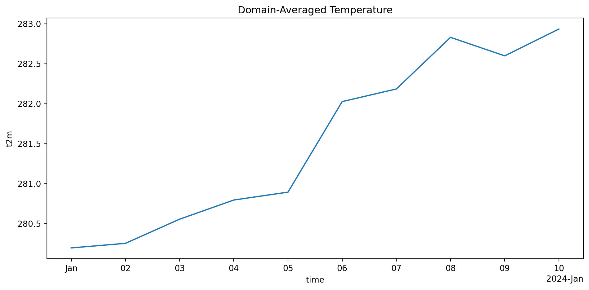
Spatially-averaged temperature (time series):
Shape: (10,)
[280.19541284 280.25248145 280.55468 280.79452266 280.89300673
282.02571815 282.18372755 282.82932531 282.59795186 282.93335992]