ATOC 4815/5815

Tabular Data & Pandas Foundations - Week 4

Will Chapman

CU Boulder ATOC

2026-01-01

Tabular Data & Pandas

Today’s Objectives

• Understanding pandas: from arrays to tables
• Reading and parsing CSV files with dates
• Time series indexing and resampling
• Rolling windows and aggregations
• Creating publication-quality time series plots
• Recognizing and fixing common pandas errors
• Building analysis workflows you’ll use in research

Reminders

Due Friday at 9pm:

• Lab 4
• HW4

Office Hours:

Will: Tu / Th 11:15-12:15p

Aiden: M / W 4-5p

The Real Problem

Your Research Scenario

Imagine: You’re analyzing Boulder’s urban heat island effect

Your data:

• 10 ASOS weather stations around Boulder
• 1 year of hourly measurements (8,760 hours × 10 stations = 87,600 rows!)
• Multiple variables: temperature, humidity, wind speed, pressure, precipitation

Each station CSV looks like:

Date and Time,Station,Temp_C,RH_pct,Wind_kt,Pressure_hPa,Precip_mm
2024-01-01 00:00,KBDU,2.1,65,8,1013.2,0.0
2024-01-01 01:00,KBDU,1.8,68,7,1013.5,0.0
2024-01-01 02:00,KBDU,1.2,71,6,1013.8,0.2
...

Questions you need to answer:

1. What’s the average daily temperature at each station?
2. Which station is warmest? When?
3. How does precipitation accumulate over the month?
4. Are there heat waves (3+ consecutive days > 30°C)?

Why NumPy Arrays Fall Short

Try solving this with NumPy arrays…

Problem 1: Multiple data types

# NumPy arrays must be uniform type
temps = np.array([2.1, 1.8, 1.2])  # ✅ Works
times = np.array(['2024-01-01 00:00', '2024-01-01 01:00'])  # ✅ Works
mixed = np.array(['KBDU', 2.1, 65])  # ❌ Everything becomes strings!

Problem 2: No column names

# How do you remember which column is which?
data = np.array([
    [2.1, 65, 8, 1013.2, 0.0],  # Station 1, hour 1
    [1.8, 68, 7, 1013.5, 0.0],  # Station 1, hour 2
])
# Is column 1 temp or humidity? Have to check your notes!

Problem 3: Time-based operations are painful

# "Give me hourly data resampled to daily" requires:
# - Manual grouping by date
# - Index math to find boundaries
# - Custom aggregation loops
# This is 20+ lines of error-prone code!

What Pandas Gives Us

Pandas solves all these problems:

1. Mixed data types in columns:

df['Station']      # Strings
df['Temp_C']       # Floats
df['Date and Time'] # Timestamps
# Each column can be different!

2. Named columns:

df['Temp_C']  # Clear what you're accessing
df['RH_pct']  # No guessing column indices

3. Time-aware operations:

# Resample hourly to daily in one line:
daily = df.resample('1D').mean()

# Rolling 24-hour average:
df['temp_24h'] = df['Temp_C'].rolling('24h').mean()

Bottom line: For tabular data with time series, Pandas is the right tool. NumPy is for uniform numeric arrays and math.

Why Pandas?

Pandas Scientific Story

Created by Wes McKinney (late 2000s) to handle panel data for quantitative finance

• Goal: bring R/Excel/SQL-style table tools into Python

Built on top of NumPy, adding:

• Labeled rows/columns (DataFrame, Series)
• Easy handling of missing values
• Powerful time-series tools (date indexes, resampling, rolling windows)

Became the standard tabular data library in scientific Python:

• Most data tutorials start with import pandas as pd
• Common front-end for reading/writing CSV, Excel, SQL, NetCDF/Parquet, etc.
• Feeds directly into NumPy, Matplotlib, and higher-level tools (xarray, geopandas, statsmodels)

For this course, think of pandas as:

“Excel + SQL + NumPy, but in code” — a single place to clean data, compute statistics, and drive time-series visualizations.

Mental Model: NumPy vs Pandas

Think of it this way:

NumPy:        "Calculator for arrays of numbers"
              ✅ Fast math, vectorized operations
              ❌ No column names, no mixed types, weak time handling

Pandas:       "Spreadsheet + database in Python"
              ✅ Named columns, mixed types, time series tools
              ✅ Built on NumPy (uses arrays internally)
              ❌ Slightly slower (but worth it for convenience)

Use NumPy when:

• Doing heavy numerical computation (matrix ops, FFT, stats)
• All data is numeric and uniform

Use Pandas when:

• Working with tables (CSV, Excel, SQL)
• Have mixed data types (strings, dates, numbers)
• Need time-based operations (resampling, rolling windows)
• Want readable code with named columns

Check Your Understanding

Which tool should you use for each task?

1. Computing the FFT of 10,000 temperature measurements

Answer: NumPy (uniform numeric array, pure math operation)

2. Loading a CSV with station names, timestamps, temps, and wind speeds

Answer: Pandas (mixed types, labeled columns, time data)

3. Calculating daily mean temperature from hourly data

Answer: Pandas (time-based resampling with .resample('1D').mean())

4. Multiplying two 1000×1000 matrices

Answer: NumPy (pure numeric computation with np.dot() or @)

Pandas Fundamentals

Series: One Column

A Series is a 1-D labeled array (like one column of a spreadsheet)

import pandas as pd
import numpy as np

# Create a Series
temps = pd.Series([15.2, 18.7, 22.1, 19.8],
                  index=['Mon', 'Tue', 'Wed', 'Thu'])
print(temps)

Mon    15.2
Tue    18.7
Wed    22.1
Thu    19.8
dtype: float64

Key features:

• .index → row labels (Mon, Tue, Wed, Thu)
• .values → underlying NumPy array
• Access by label: temps['Mon'] → 15.2
• Access by position: temps[0] → 15.2

DataFrame: Multiple Series

A DataFrame is a 2-D table (like a whole spreadsheet)

# Create a DataFrame
data = pd.DataFrame({
    'temp_c': [15.2, 18.7, 22.1, 19.8],
    'pressure_hpa': [1010, 1012, 1008, 1011]
}, index=['Mon', 'Tue', 'Wed', 'Thu'])
print(data)

     temp_c  pressure_hpa
Mon    15.2          1010
Tue    18.7          1012
Wed    22.1          1008
Thu    19.8          1011

Key features:

• .columns → column names (temp_c, pressure_hpa)
• .index → row labels (Mon, Tue, Wed, Thu)
• Each column is a Series
• Access column: data['temp_c'] → Series
• Access row: data.loc['Mon'] → Series

Common Error: Accessing Columns

Predict the output:

import pandas as pd

df = pd.DataFrame({
    'temp_c': [15.2, 18.7, 22.1],
    'station': ['KBDU', 'KDEN', 'KBJC']
})

print(df.temp_c)  # Does this work?

0    15.2
1    18.7
2    22.1
Name: temp_c, dtype: float64

✅ It works! But there’s a catch…

The Problem:

# ✅ Good: Always use bracket notation
df['temp_c']

# ⚠️ Risky: Dot notation fails if column name has spaces or conflicts
df.temp c      # SyntaxError!
df.max         # Gets the method, not a column named 'max'!

Best practice: Always use df['column_name'] for columns

Common Error: KeyError

Predict the output:

df = pd.DataFrame({
    'temp_c': [15.2, 18.7, 22.1],
    'station': ['KBDU', 'KDEN', 'KBJC']
})

print(df['temperature'])  # What happens?

KeyError: 'temperature'

Explanation: Column ‘temperature’ doesn’t exist (it’s ‘temp_c’)

The Fix:

# Check available columns first
print(df.columns)  # Index(['temp_c', 'station'], dtype='object')

# Or use .get() with a default
value = df.get('temperature', default=None)  # Returns None instead of error

Common causes:

• Typo in column name
• Wrong capitalization (‘Temp_C’ vs ‘temp_c’)
• Column was renamed or not read from CSV

Try It Yourself 💻

With your neighbor (3 min): Create a DataFrame with Boulder weather

weather = pd.DataFrame({
    'date': ['2024-01-01', '2024-01-02', '2024-01-03'],
    'temp_c': [2.1, 3.5, 1.2],
    'precip_mm': [0.0, 2.5, 0.5]
})

# Tasks:
# 1. Print the DataFrame
# 2. Extract just the temp_c column
# 3. What's the maximum precipitation?
# 4. Try accessing a column that doesn't exist—what error do you get?

Answers:

# 1.
print(weather)

# 2.
temps = weather['temp_c']

# 3.
max_precip = weather['precip_mm'].max()  # 2.5

# 4.
weather['humidity']  # KeyError: 'humidity'

Reading Data

Reading CSVs: The Wrong Way

What happens if you just read the CSV naively?

# Sample CSV as a string (simulating a file)
import io
csv_data = """Date and Time,Station,Temp_C
2024-01-01 00:00,KBDU,2.1
2024-01-01 01:00,KBDU,1.8
2024-01-01 02:00,KBDU,1.2"""

df_wrong = pd.read_csv(io.StringIO(csv_data))
print(df_wrong)
print(f"\nData type of 'Date and Time': {df_wrong['Date and Time'].dtype}")

      Date and Time Station  Temp_C
0  2024-01-01 00:00    KBDU     2.1
1  2024-01-01 01:00    KBDU     1.8
2  2024-01-01 02:00    KBDU     1.2

Data type of 'Date and Time': object

Problem: ‘Date and Time’ is stored as a string (object), not a timestamp!

Why it matters:

• Can’t do time-based operations (resampling, rolling windows)
• Can’t filter by date easily
• Can’t extract month, day, hour

Reading CSVs: The Right Way

Use parse_dates to convert string → datetime:

csv_data = """Date and Time,Station,Temp_C
2024-01-01 00:00,KBDU,2.1
2024-01-01 01:00,KBDU,1.8
2024-01-01 02:00,KBDU,1.2"""

df_right = pd.read_csv(io.StringIO(csv_data), parse_dates=['Date and Time'])
print(df_right)
print(f"\nData type of 'Date and Time': {df_right['Date and Time'].dtype}")

        Date and Time Station  Temp_C
0 2024-01-01 00:00:00    KBDU     2.1
1 2024-01-01 01:00:00    KBDU     1.8
2 2024-01-01 02:00:00    KBDU     1.2

Data type of 'Date and Time': datetime64[ns]

Now it’s a datetime64 type!

What you can do now:

# Extract components
print(f"Hour of first row: {df_right['Date and Time'][0].hour}")

# Filter by date
after_midnight = df_right[df_right['Date and Time'] >= '2024-01-01 01:00']
print(f"\nRows after midnight: {len(after_midnight)}")

Hour of first row: 0

Rows after midnight: 2

Common Error: Forgetting parse_dates

Predict the output:

# CSV read WITHOUT parse_dates
df = pd.read_csv('weather.csv')  # Forgot parse_dates!

# Try to resample to daily
daily = df.resample('1D').mean()

TypeError: Only valid with DatetimeIndex, TimedeltaIndex or PeriodIndex,
but got an instance of 'RangeIndex'

Explanation: Can’t resample without a time index!

The Fix:

# Method 1: Parse on read
df = pd.read_csv('weather.csv', parse_dates=['Date and Time'])
df = df.set_index('Date and Time')
daily = df.resample('1D').mean()  # ✅ Works!

# Method 2: Convert after reading
df = pd.read_csv('weather.csv')
df['Date and Time'] = pd.to_datetime(df['Date and Time'])
df = df.set_index('Date and Time')

Setting a Time Index

For time series analysis, make the timestamp the index

Why?

• Enables .resample(), .rolling(), time-based slicing
• Aligns operations by time automatically
• Makes plots use time on x-axis by default

# Create sample data
dates = pd.date_range('2024-01-01', periods=5, freq='h')
df = pd.DataFrame({
    'temp_c': [15.2, 16.1, 17.3, 18.2, 17.5],
    'pressure_hpa': [1010, 1011, 1009, 1008, 1010]
}, index=dates)

print(df)
print(f"\nIndex type: {type(df.index)}")

                     temp_c  pressure_hpa
2024-01-01 00:00:00    15.2          1010
2024-01-01 01:00:00    16.1          1011
2024-01-01 02:00:00    17.3          1009
2024-01-01 03:00:00    18.2          1008
2024-01-01 04:00:00    17.5          1010

Index type: <class 'pandas.core.indexes.datetimes.DatetimeIndex'>

Now time-based operations work:

# Time-based slicing
print("\n2-hour window:")
print(df['2024-01-01 02:00':'2024-01-01 04:00'])

2-hour window:
                     temp_c  pressure_hpa
2024-01-01 02:00:00    17.3          1009
2024-01-01 03:00:00    18.2          1008
2024-01-01 04:00:00    17.5          1010

Setting Index: Two Methods

Method 1: Set index after reading

df = pd.read_csv('weather.csv', parse_dates=['Date and Time'])
df = df.set_index('Date and Time')

Method 2: Set index during read (more efficient)

df = pd.read_csv('weather.csv',
                 parse_dates=['Date and Time'],
                 index_col='Date and Time')

Method 2 is better:

• One step instead of two
• Slightly faster (one less copy)
• Less code to maintain

Check Your Understanding

What’s wrong with this code?

df = pd.read_csv('boulder_weather.csv')
daily_mean = df.resample('1D').mean()

Two problems:

1. ❌ No parse_dates — dates are strings, not datetimes
2. ❌ No time index set — can’t resample without DatetimeIndex

The fix:

df = pd.read_csv('boulder_weather.csv',
                 parse_dates=['Date and Time'],
                 index_col='Date and Time')
daily_mean = df.resample('1D').mean()  # ✅ Now it works!

Resampling & Aggregation

What is Resampling?

Resampling: Change the frequency of your time series

Visual example:

Hourly data (24 points per day):
├─ 00:00 → 15.2°C
├─ 01:00 → 16.1°C
├─ 02:00 → 17.3°C
├─ 03:00 → 18.2°C
   ...

Resample to daily (1 point per day):
└─ 2024-01-01 → 16.7°C (mean of all 24 hours)

Common patterns:

• Downsampling: High → Low frequency (hourly → daily)
• Aggregation: How to combine values (mean, sum, max, min, etc.)

Resampling Syntax

# Create 15-minute data
dates = pd.date_range('2024-01-01', periods=96, freq='15min')
df = pd.DataFrame({
    'temp_c': 15 + 5 * np.sin(np.arange(96) * 2 * np.pi / 96) + np.random.randn(96) * 0.5,
    'precip_mm': np.random.exponential(0.1, 96)
}, index=dates)

print("Original (15-min):")
print(df.head())

# Resample to hourly
hourly = df.resample('1h').mean()

print("\nResampled (hourly):")
print(hourly.head())

Original (15-min):
                        temp_c  precip_mm
2024-01-01 00:00:00  16.173676   0.099685
2024-01-01 00:15:00  14.848665   0.081673
2024-01-01 00:30:00  16.194610   0.079385
2024-01-01 00:45:00  16.101159   0.068615
2024-01-01 01:00:00  16.407122   0.167338

Resampled (hourly):
                        temp_c  precip_mm
2024-01-01 00:00:00  15.829528   0.082339
2024-01-01 01:00:00  16.836664   0.105572
2024-01-01 02:00:00  18.503434   0.106796
2024-01-01 03:00:00  19.021177   0.190675
2024-01-01 04:00:00  19.634585   0.175629

Aggregation Rules: When to Use What?

Different variables need different aggregation methods:

Variable	Aggregation	Why?
Temperature	mean()	Average temp over period makes sense
Precipitation	sum()	Want total accumulated precip
Wind speed	mean() or max()	Mean for typical, max for gusts
Pressure	mean()	Average pressure over period
Station ID	first()	Metadata—just keep one

Example:

# Different rules for different columns
hourly = df.resample('1h').agg({
    'temp_c': 'mean',      # Average temperature
    'precip_mm': 'sum'     # Total precipitation
})

print(hourly.head(3))

                        temp_c  precip_mm
2024-01-01 00:00:00  15.829528   0.329358
2024-01-01 01:00:00  16.836664   0.422289
2024-01-01 02:00:00  18.503434   0.427185

Common Error: Wrong Aggregation

Predict the problem:

# 24 hours of precipitation data
precip = pd.Series([0.5, 0.2, 0.0, 0.8, ...], index=hourly_times)

# Resample to daily
daily_precip = precip.resample('1D').mean()  # ❌ WRONG!

The Problem: Using mean() for precipitation!

• You don’t want the “average hourly precip”
• You want “total daily precip”

The Fix:

daily_precip = precip.resample('1D').sum()  # ✅ Correct!

Example:

Hourly:  [0.5, 0.2, 0.0, 0.8] mm
Daily (wrong): mean = 0.375 mm  ← What does this even mean?
Daily (right): sum = 1.5 mm      ← Total precip for the day

Try It Yourself 💻

With your neighbor (5 min): Practice resampling

# Create hourly temperature data
dates = pd.date_range('2024-01-01', periods=168, freq='h')  # 1 week
temps = pd.Series(
    15 + 8 * np.sin(np.arange(168) * 2 * np.pi / 24) + np.random.randn(168),
    index=dates
)

# Tasks:
# 1. Resample to daily mean temperature
# 2. Find the warmest day
# 3. Resample to 6-hour max temperature
# 4. What happens if you resample but forget to call .mean() or .sum()?

Answers:

# 1. Daily mean
daily = temps.resample('1D').mean()

# 2. Warmest day
warmest = daily.idxmax()  # Returns the date
print(f"Warmest day: {warmest} at {daily.max():.1f}°C")

# 3. 6-hour max
six_hour_max = temps.resample('6h').max()

# 4. Forget aggregation
resampled = temps.resample('1D')  # Just returns a Resampler object, not data!
print(resampled)  # DatetimeIndexResampler [freq=<Day>, ...]

Multiple Aggregations

You can compute multiple statistics at once:

# Create sample data
dates = pd.date_range('2024-01-01', periods=168, freq='h')
df = pd.DataFrame({
    'temp_c': 15 + 8 * np.sin(np.arange(168) * 2 * np.pi / 24) + np.random.randn(168) * 2,
    'precip_mm': np.random.exponential(0.3, 168)
}, index=dates)

# Daily aggregation with different rules
daily = df.resample('1D').agg({
    'temp_c': ['mean', 'min', 'max'],
    'precip_mm': 'sum'
})

print(daily)

               temp_c                      precip_mm
                 mean       min        max       sum
2024-01-01  14.259125  5.390141  25.209704  6.751797
2024-01-02  15.005423  3.997170  27.767386  5.536288
2024-01-03  14.646785  5.440125  25.165309  9.582820
2024-01-04  14.406230  5.744967  24.143758  7.282788
2024-01-05  15.251515  4.546007  26.057174  4.198441
2024-01-06  14.316535  5.084648  24.766982  9.007464
2024-01-07  14.880477  5.357552  26.838364  6.845535

Accessing multi-level columns:

# Access specific aggregation
daily_mean_temp = daily['temp_c']['mean']
daily_precip = daily['precip_mm']['sum']

print(f"\nFirst day mean temp: {daily_mean_temp.iloc[0]:.1f}°C")
print(f"First day total precip: {daily_precip.iloc[0]:.2f} mm")

First day mean temp: 14.3°C
First day total precip: 6.75 mm

Resampling Frequency Codes

Common frequency strings:

Code	Meaning	Example
'1h'	Hourly	Every hour
'3h'	Every 3 hours	00:00, 03:00, 06:00, …
'1D'	Daily	Once per day
'1W'	Weekly	Once per week
'1MS'	Monthly (start)	First day of each month
'1ME'	Monthly (end)	Last day of each month
'1QS'	Quarterly (start)	Jan 1, Apr 1, Jul 1, Oct 1
'1YS'	Yearly (start)	Jan 1 each year

You can combine numbers and codes:

df.resample('6h').mean()    # Every 6 hours
df.resample('15min').sum()  # Every 15 minutes
df.resample('2W').max()     # Every 2 weeks

Check Your Understanding

For each scenario, which aggregation should you use?

1. Converting hourly temperature to daily

Answer: mean() — average temperature for the day

2. Converting 5-minute rainfall to hourly

Answer: sum() — total rainfall accumulated per hour

3. Converting hourly wind speed to daily

Answer: Could use mean() for typical wind, or max() for peak gusts

4. Converting hourly pressure to 6-hour

Answer: mean() — average pressure over 6-hour period

Rolling Windows

What is a Rolling Window?

Rolling window: Compute statistics over a moving time window

Visual example:

Data:     [10, 12, 15, 18, 20, 22, 21, 19, 16, 14]
           ↓   ↓   ↓
Window:   [10, 12, 15]  → mean = 12.3
               ↓   ↓   ↓
Window:       [12, 15, 18]  → mean = 15.0
                   ↓   ↓   ↓
Window:           [15, 18, 20]  → mean = 17.7
                       ...

Result: A smoothed version of the original data

Rolling Window Syntax

# Create hourly temperature data
dates = pd.date_range('2024-01-01', periods=168, freq='h')
temps = pd.Series(
    15 + 8 * np.sin(np.arange(168) * 2 * np.pi / 24) + np.random.randn(168) * 2,
    index=dates
)

# Rolling means with different windows
temps_3h = temps.rolling('3h').mean()
temps_12h = temps.rolling('12h').mean()
temps_24h = temps.rolling('24h').mean()

print("Original vs Rolling means:")
df_compare = pd.DataFrame({
    'original': temps,
    'rolling_3h': temps_3h,
    'rolling_12h': temps_12h,
    'rolling_24h': temps_24h
})
print(df_compare.head(26))

Original vs Rolling means:
                      original  rolling_3h  rolling_12h  rolling_24h
2024-01-01 00:00:00  14.889767   14.889767    14.889767    14.889767
2024-01-01 01:00:00  15.790868   15.340317    15.340317    15.340317
2024-01-01 02:00:00  19.000372   16.560336    16.560336    16.560336
2024-01-01 03:00:00  20.295435   18.362225    17.494110    17.494110
2024-01-01 04:00:00  19.301853   19.532553    17.855659    17.855659
2024-01-01 05:00:00  24.996085   21.531124    19.045730    19.045730
2024-01-01 06:00:00  25.609007   23.302315    19.983341    19.983341
2024-01-01 07:00:00  21.909126   24.171406    20.224064    20.224064
2024-01-01 08:00:00  23.679977   23.732703    20.608054    20.608054
2024-01-01 09:00:00  22.319090   22.636064    20.779158    20.779158
2024-01-01 10:00:00  22.778157   22.925741    20.960885    20.960885
2024-01-01 11:00:00  15.643745   20.246997    20.517790    20.517790
2024-01-01 12:00:00  13.582830   17.334911    20.408879    19.984332
2024-01-01 13:00:00  15.687270   14.971282    20.400246    19.677399
2024-01-01 14:00:00   8.446805   12.572302    19.520782    18.928692
2024-01-01 15:00:00   4.226297    9.453458    18.181687    18.009793
2024-01-01 16:00:00   8.362941    7.012014    17.270111    17.442331
2024-01-01 17:00:00   9.153012    7.247417    15.949855    16.981813
2024-01-01 18:00:00   9.259211    8.925055    14.587372    16.575360
2024-01-01 19:00:00   8.970876    9.127700    13.509184    16.195136
2024-01-01 20:00:00   7.860450    8.696846    12.190890    15.798246
2024-01-01 21:00:00   6.703500    7.844942    10.889591    15.384849
2024-01-01 22:00:00   8.621854    7.728601     9.709899    15.090806
2024-01-01 23:00:00  12.131319    9.152224     9.417197    14.967494
2024-01-02 00:00:00  17.388139   12.713771     9.734306    15.071592
2024-01-02 01:00:00  17.508724   15.676061     9.886094    15.143170

Rolling Window Visualization

import matplotlib.pyplot as plt

# Plot raw data and rolling means
plt.figure(figsize=(9, 4))
plt.plot(temps.index, temps, alpha=0.3, label='Raw (hourly)', linewidth=1)
plt.plot(temps.index, temps_3h, label='3-hour rolling mean', linewidth=1.5)
plt.plot(temps.index, temps_12h, label='12-hour rolling mean', linewidth=1.5)
plt.plot(temps.index, temps_24h, label='24-hour rolling mean', linewidth=2)
plt.xlabel('Date')
plt.ylabel('Temperature (°C)')
plt.title('Temperature with Rolling Means')
plt.legend()
plt.grid(True, alpha=0.3)
plt.tight_layout()
plt.show()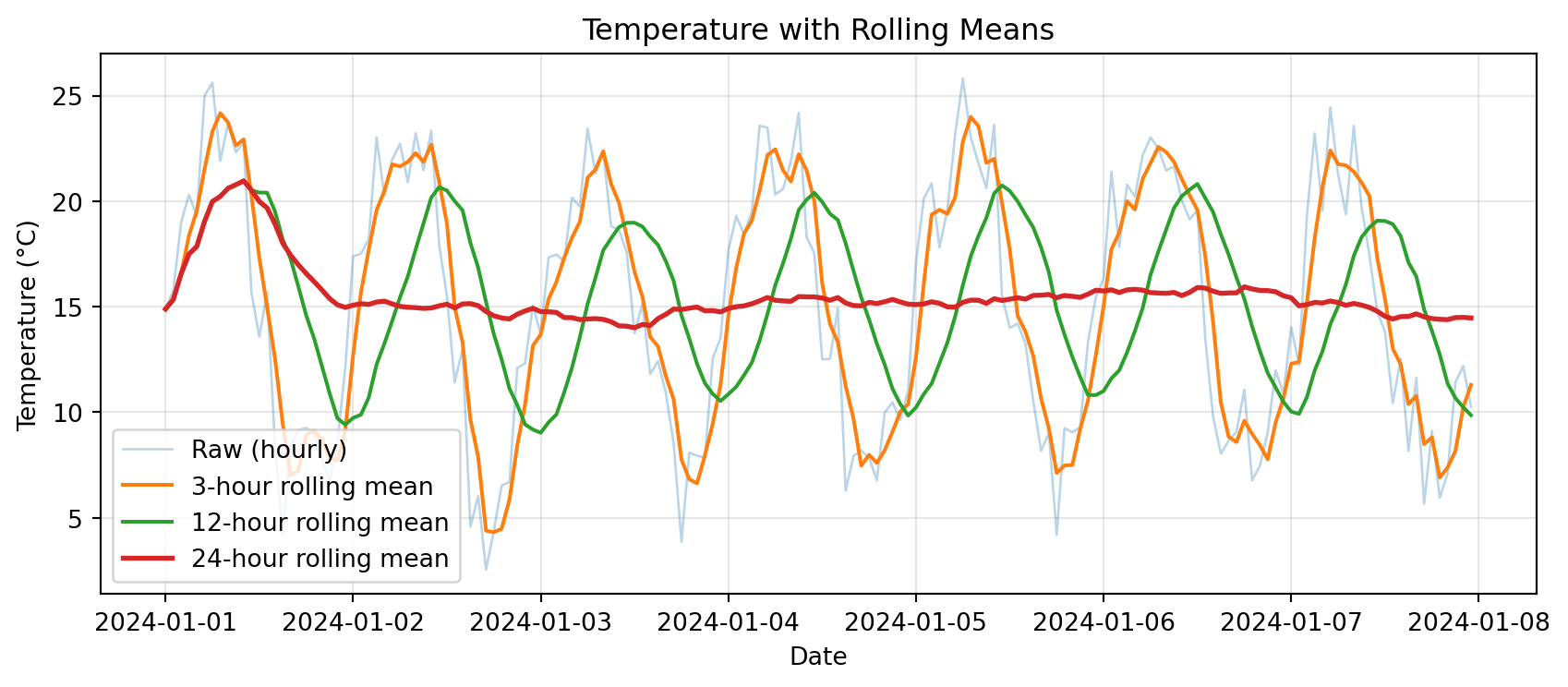

Notice: Longer windows → smoother curves, but more lag

Rolling vs Resampling: What’s the Difference?

Resampling: Change frequency (hourly → daily)

• Reduces number of points
• Each point represents a whole period

Rolling: Smooth data over a moving window

• Same number of points (except edge NaNs)
• Each point is an average of nearby points

Example:

# Original: 168 hourly points
print(f"Original: {len(temps)} points")

# Resampling to daily: reduces to 7 points
daily = temps.resample('1D').mean()
print(f"Resampled daily: {len(daily)} points")

# Rolling 24-hour: still 168 points (but first 23 are NaN)
rolling_24h = temps.rolling('24h').mean()
print(f"Rolling 24h: {len(rolling_24h)} points (includes NaN at start)")

Original: 168 points
Resampled daily: 7 points
Rolling 24h: 168 points (includes NaN at start)

Common Error: Rolling on Wrong Data Type

Predict the output:

df = pd.DataFrame({
    'station': ['KBDU', 'KBDU', 'KBDU', 'KBDU'],
    'temp_c': [15.2, 16.1, 17.3, 18.2]
})

# Try rolling mean on station names
rolling = df['station'].rolling(3).mean()

TypeError: unsupported operand type(s) for /: 'str' and 'int'

Explanation: Can’t compute mean of strings!

The Fix:

# ✅ Rolling on numeric data
rolling = df['temp_c'].rolling(3).mean()

# ✅ Or select numeric columns only
rolling = df.select_dtypes(include=[np.number]).rolling(3).mean()

Rolling Statistics Beyond Mean

Rolling windows aren’t just for means:

# Create temperature data
dates = pd.date_range('2024-01-01', periods=168, freq='h')
temps = pd.Series(
    15 + 8 * np.sin(np.arange(168) * 2 * np.pi / 24) + np.random.randn(168) * 2,
    index=dates
)

# Different rolling statistics
rolling_mean = temps.rolling('24h').mean()
rolling_std = temps.rolling('24h').std()
rolling_min = temps.rolling('24h').min()
rolling_max = temps.rolling('24h').max()

print("Rolling 24-hour statistics:")
print(pd.DataFrame({
    'mean': rolling_mean,
    'std': rolling_std,
    'min': rolling_min,
    'max': rolling_max
}).describe())

Rolling 24-hour statistics:
             mean         std         min         max
count  168.000000  167.000000  168.000000  168.000000
mean    15.668326    5.941928    6.629573   25.198995
std      1.412319    1.091453    3.200625    1.543924
min     14.586066    0.257213    4.250910   17.820791
25%     15.013856    5.889691    4.940989   24.260239
50%     15.219206    6.244654    6.211150   25.254050
75%     15.557183    6.453377    6.341110   25.962735
max     21.297948    7.095308   17.820791   27.930284

Use Case: Temperature Variability

Rolling standard deviation shows how variable conditions are:

# Create data with changing variability
dates = pd.date_range('2024-01-01', periods=168, freq='h')
# Add more noise in second half
noise = np.concatenate([
    np.random.randn(84) * 1,    # Low variability
    np.random.randn(84) * 4     # High variability
])
temps = pd.Series(
    15 + 8 * np.sin(np.arange(168) * 2 * np.pi / 24) + noise,
    index=dates
)

rolling_mean = temps.rolling('12h').mean()
rolling_std = temps.rolling('12h').std()

# Plot
fig, (ax1, ax2) = plt.subplots(2, 1, figsize=(9, 5), sharex=True)

ax1.plot(temps.index, temps, alpha=0.4, label='Hourly temp')
ax1.plot(temps.index, rolling_mean, linewidth=2, label='12-h mean')
ax1.set_ylabel('Temperature (°C)')
ax1.set_title('Temperature and Variability')
ax1.legend()
ax1.grid(True, alpha=0.3)

ax2.plot(temps.index, rolling_std, color='red', linewidth=2)
ax2.set_xlabel('Date')
ax2.set_ylabel('Rolling Std Dev (°C)')
ax2.set_title('12-hour Rolling Variability')
ax2.grid(True, alpha=0.3)

plt.tight_layout()
plt.show()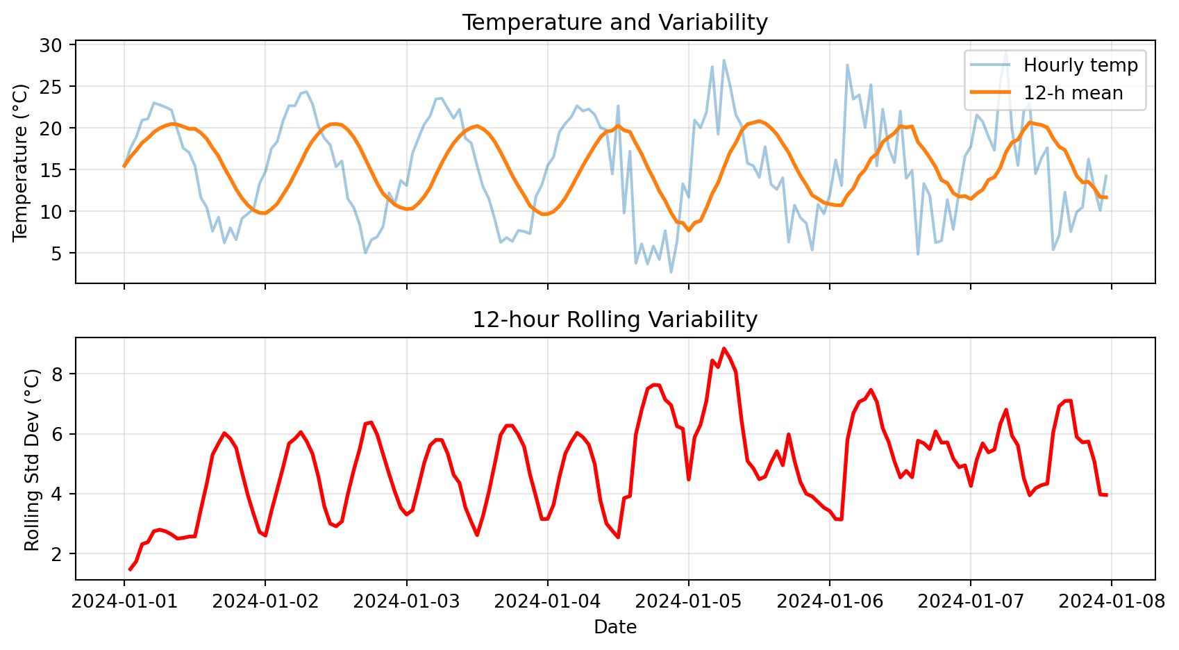

Notice: High rolling std in second half → more variable conditions

Try It Yourself 💻

With your neighbor (5 min): Explore rolling windows

# Create 1 week of hourly wind speed data
dates = pd.date_range('2024-01-01', periods=168, freq='h')
wind_kt = pd.Series(
    10 + 5 * np.abs(np.sin(np.arange(168) * 2 * np.pi / 24)) + np.random.randn(168) * 2,
    index=dates
)

# Tasks:
# 1. Compute 6-hour rolling mean wind speed
# 2. Find the time period with highest 6-hour average wind
# 3. Compute 12-hour rolling max (for peak gusts)
# 4. What's the difference between .rolling(6) and .rolling('6h')?

Answers:

# 1. 6-hour rolling mean
rolling_mean_6h = wind_kt.rolling('6h').mean()

# 2. Highest 6-hour average
max_time = rolling_mean_6h.idxmax()
max_wind = rolling_mean_6h.max()
print(f"Highest 6-h avg wind: {max_wind:.1f} kt at {max_time}")

# 3. 12-hour rolling max
rolling_max_12h = wind_kt.rolling('12h').max()

# 4. Difference:
# .rolling(6) → 6 data points (may not be 6 hours if data is irregular)
# .rolling('6h') → 6 hours of data (time-aware, handles gaps correctly)

Anomalies & Cumulative Sums

Computing Anomalies

Anomaly: Deviation from a baseline (climatology, daily mean, etc.)

Why anomalies matter:

• Identify unusual events
• Remove seasonal cycle
• Compare different stations or years

Example: Hourly temperature anomalies from daily mean

# Create hourly data for a week
dates = pd.date_range('2024-01-01', periods=168, freq='h')
temps = pd.Series(
    15 + 8 * np.sin(np.arange(168) * 2 * np.pi / 24) + np.random.randn(168) * 2,
    index=dates
)
df = pd.DataFrame({'temp_c': temps})

# Method: use groupby to compute daily mean, then subtract
df['date'] = df.index.date
df['daily_mean'] = df.groupby('date')['temp_c'].transform('mean')
df['anomaly'] = df['temp_c'] - df['daily_mean']

print(df[['temp_c', 'daily_mean', 'anomaly']].head(10))

                        temp_c  daily_mean   anomaly
2024-01-01 00:00:00  15.974748     15.1421  0.832647
2024-01-01 01:00:00  17.535899     15.1421  2.393799
2024-01-01 02:00:00  20.237654     15.1421  5.095554
2024-01-01 03:00:00  20.716450     15.1421  5.574349
2024-01-01 04:00:00  22.439275     15.1421  7.297175
2024-01-01 05:00:00  22.054399     15.1421  6.912298
2024-01-01 06:00:00  22.186110     15.1421  7.044009
2024-01-01 07:00:00  22.802955     15.1421  7.660855
2024-01-01 08:00:00  19.359851     15.1421  4.217750
2024-01-01 09:00:00  19.641332     15.1421  4.499232

Visualizing Anomalies

# Plot raw data and anomalies
fig, (ax1, ax2) = plt.subplots(2, 1, figsize=(9, 5), sharex=True)

# Top: Raw temperature
ax1.plot(df.index, df['temp_c'], label='Hourly temp', alpha=0.7)
ax1.plot(df.index, df['daily_mean'], label='Daily mean', linewidth=2, color='red')
ax1.set_ylabel('Temperature (°C)')
ax1.set_title('Raw Temperature and Daily Mean')
ax1.legend()
ax1.grid(True, alpha=0.3)

# Bottom: Anomalies
ax2.plot(df.index, df['anomaly'], color='purple', alpha=0.7)
ax2.axhline(y=0, color='black', linestyle='--', linewidth=1)
ax2.set_xlabel('Date')
ax2.set_ylabel('Anomaly (°C)')
ax2.set_title('Hourly Anomalies from Daily Mean')
ax2.grid(True, alpha=0.3)

plt.tight_layout()
plt.show()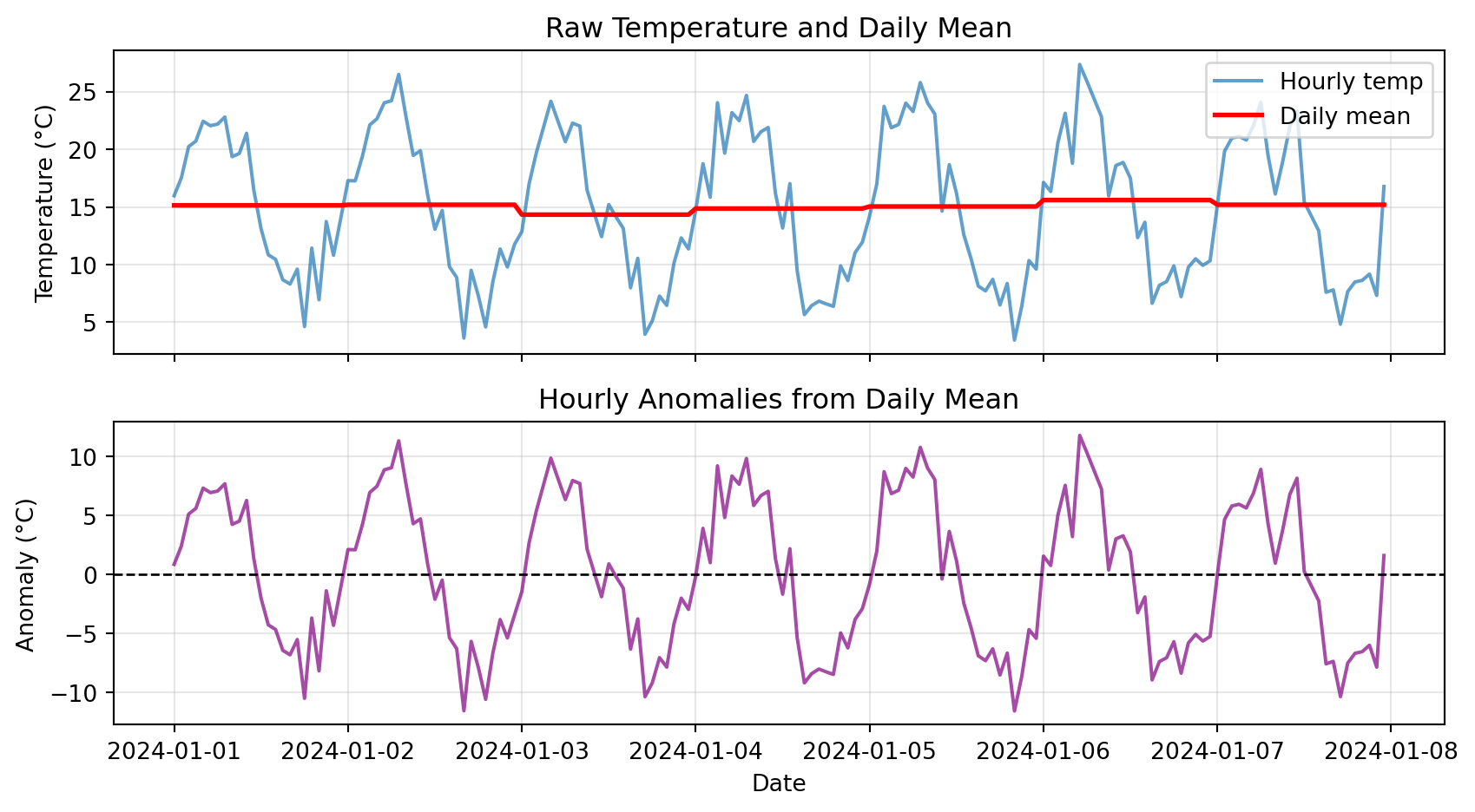

Notice: Anomalies oscillate around zero, showing deviations from typical pattern

Cumulative Sums

Cumulative sum: Running total over time

Use cases:

• Precipitation: Total accumulated rainfall
• Energy: Cumulative power consumption
• Degree-days: Accumulated heat or cold

# Create precipitation data
dates = pd.date_range('2024-01-01', periods=168, freq='h')
precip = pd.Series(np.random.exponential(0.3, 168), index=dates)

# Compute cumulative sum
cumulative = precip.cumsum()

print("Hourly and cumulative precipitation:")
print(pd.DataFrame({
    'hourly_mm': precip,
    'cumulative_mm': cumulative
}).head(10))

Hourly and cumulative precipitation:
                     hourly_mm  cumulative_mm
2024-01-01 00:00:00   0.059461       0.059461
2024-01-01 01:00:00   0.185887       0.245348
2024-01-01 02:00:00   0.114193       0.359542
2024-01-01 03:00:00   1.110091       1.469633
2024-01-01 04:00:00   0.058819       1.528451
2024-01-01 05:00:00   0.265696       1.794147
2024-01-01 06:00:00   0.269267       2.063414
2024-01-01 07:00:00   0.851558       2.914972
2024-01-01 08:00:00   0.090930       3.005902
2024-01-01 09:00:00   0.361807       3.367708

Cumulative Precipitation Visualization

# Plot hourly and cumulative
fig, (ax1, ax2) = plt.subplots(2, 1, figsize=(9, 5), sharex=True)

# Top: Hourly bars
ax1.bar(precip.index, precip, width=0.04, alpha=0.6, color='steelblue')
ax1.set_ylabel('Hourly Precip (mm)')
ax1.set_title('Hourly Precipitation')
ax1.grid(True, alpha=0.3)

# Bottom: Cumulative line
ax2.plot(cumulative.index, cumulative, linewidth=2, color='darkblue')
ax2.set_xlabel('Date')
ax2.set_ylabel('Cumulative Precip (mm)')
ax2.set_title('Cumulative Precipitation')
ax2.grid(True, alpha=0.3)

plt.tight_layout()
plt.show()

print(f"\nTotal precipitation over week: {cumulative.iloc[-1]:.2f} mm")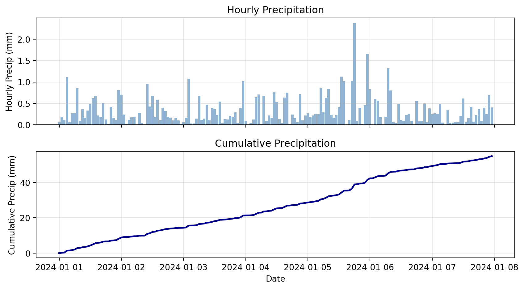

Total precipitation over week: 54.87 mm

Check Your Understanding

Match each technique to its use case:

Techniques:

1. Rolling mean
2. Resampling
3. Anomaly
4. Cumulative sum

Use cases:

A. “How much total rainfall since Jan 1?”

B. “What’s the smoothed temperature trend?”

C. “Convert hourly data to daily averages”

D. “How much warmer than normal was today?”

Answers:

1-B (Rolling mean → smoothing)

2-C (Resampling → change frequency)

3-D (Anomaly → deviation from baseline)

4-A (Cumulative sum → total accumulated)

Plotting Time Series

Pandas Native Plotting

Pandas DataFrames have built-in .plot() method:

# Create sample data
dates = pd.date_range('2024-01-01', periods=168, freq='h')
df_plot = pd.DataFrame({
    'temp_c': 15 + 8 * np.sin(np.arange(168) * 2 * np.pi / 24) + np.random.randn(168) * 2,
}, index=dates)
df_plot['rolling_24h'] = df_plot['temp_c'].rolling('24h').mean()

# Simple plot
df_plot.plot(
    figsize=(9, 4),
    title='Temperature Time Series',
    ylabel='Temperature (°C)',
    grid=True,
    alpha=0.7
)
plt.tight_layout()
plt.show()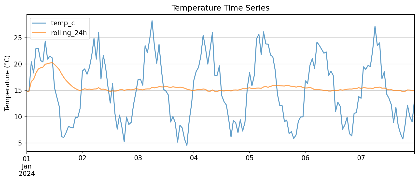

Key advantage: .plot() automatically uses the index as x-axis

Multi-Panel Time Series

For complex analysis, use matplotlib subplots:

# Create comprehensive dataset
dates = pd.date_range('2024-01-01', periods=168, freq='h')
weather = pd.DataFrame({
    'temp_c': 15 + 8 * np.sin(np.arange(168) * 2 * np.pi / 24) + np.random.randn(168) * 2,
    'rh_pct': 60 + 20 * np.sin(np.arange(168) * 2 * np.pi / 24 + np.pi/4) + np.random.randn(168) * 5,
    'precip_mm': np.random.exponential(0.3, 168)
}, index=dates)

# Add derived quantities
weather['temp_rolling_24h'] = weather['temp_c'].rolling('24h').mean()
weather['cumulative_precip'] = weather['precip_mm'].cumsum()

# Create multi-panel plot
fig, (ax1, ax2, ax3) = plt.subplots(3, 1, figsize=(9, 7), sharex=True)

# Panel 1: Temperature
ax1.plot(weather.index, weather['temp_c'], alpha=0.4, label='Hourly Temp')
ax1.plot(weather.index, weather['temp_rolling_24h'], linewidth=2, label='24-h Rolling Mean')
ax1.set_ylabel('Temperature (°C)')
ax1.set_title('Weather Time Series Analysis')
ax1.legend(loc='best')
ax1.grid(True, alpha=0.3)

# Panel 2: Relative Humidity
ax2.plot(weather.index, weather['rh_pct'], color='green', alpha=0.7)
ax2.set_ylabel('Relative Humidity (%)')
ax2.grid(True, alpha=0.3)

# Panel 3: Precipitation (dual y-axes)
ax3.bar(weather.index, weather['precip_mm'], width=0.04, alpha=0.6, label='Hourly Precip')
ax3_cum = ax3.twinx()
ax3_cum.plot(weather.index, weather['cumulative_precip'], color='steelblue',
             linewidth=2, label='Cumulative')
ax3.set_xlabel('Date')
ax3.set_ylabel('Hourly Precip (mm)')
ax3_cum.set_ylabel('Cumulative (mm)')
ax3.legend(loc='upper left')
ax3_cum.legend(loc='upper right')
ax3.grid(True, alpha=0.3)

plt.tight_layout()
plt.show()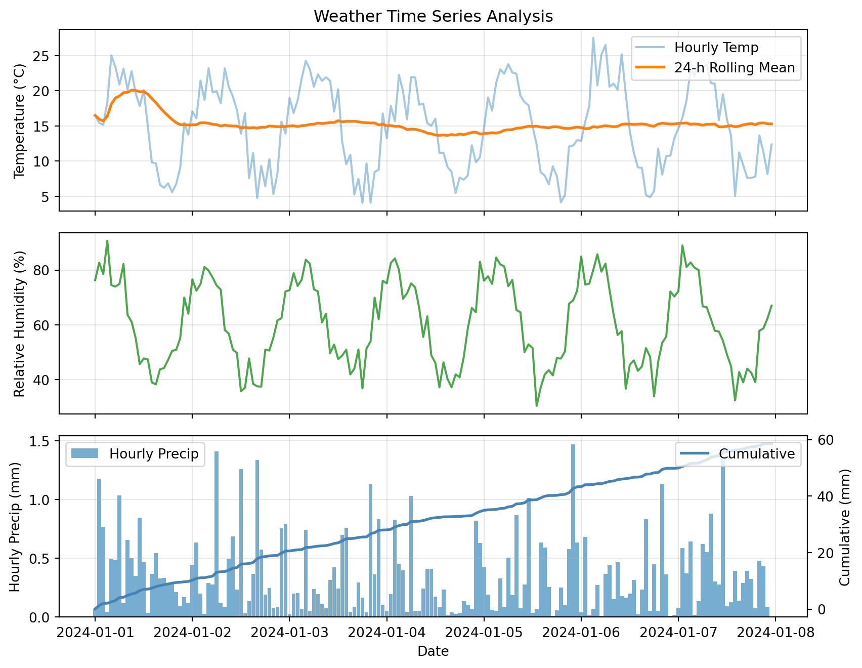

This plot combines:

• Raw and smoothed time series (top)
• Secondary variables (middle)
• Dual y-axes for different scales (bottom)

Advanced Topics

Boolean Filtering with Time Index

With a time index, boolean masks work just like NumPy:

# Create precipitation data
dates = pd.date_range('2024-01-01', periods=168, freq='h')
precip_df = pd.DataFrame({
    'precip_mm': np.random.exponential(0.3, 168)
}, index=dates)

# Boolean mask: rainy hours (> 0.5 mm)
rainy_hours = precip_df['precip_mm'] > 0.5

# Count and extract
print(f"Number of rainy hours: {rainy_hours.sum()}")
print(f"\nRainiest hours:")
print(precip_df[rainy_hours].nlargest(5, 'precip_mm'))

Number of rainy hours: 33

Rainiest hours:
                     precip_mm
2024-01-05 19:00:00   1.203417
2024-01-06 08:00:00   1.097777
2024-01-04 05:00:00   1.078415
2024-01-03 00:00:00   1.023506
2024-01-03 23:00:00   1.016585

Combine conditions:

# Hot and dry conditions
hot_dry = (weather['temp_c'] > 30) & (weather['rh_pct'] < 20)

# Cold or very wet
cold_wet = (weather['temp_c'] < 0) | (weather['precip_mm'] > 5)

Helper Functions for Reusable Analysis

Instead of copy-pasting analysis code, wrap it in functions:

def summarize_period(df, freq='1D', temp_col='temp_c', precip_col='precip_mm'):
    """
    Resample time series to specified frequency.

    Parameters
    ----------
    df : pd.DataFrame
        Input dataframe with time index
    freq : str
        Resample frequency ('1h', '1D', '1W', etc.)
    temp_col : str
        Name of temperature column
    precip_col : str
        Name of precipitation column

    Returns
    -------
    pd.DataFrame
        Resampled data with mean temp and total precip
    """
    # Check that required columns exist
    if temp_col not in df.columns:
        raise ValueError(f"Column '{temp_col}' not found in DataFrame")
    if precip_col not in df.columns:
        raise ValueError(f"Column '{precip_col}' not found in DataFrame")

    # Resample with appropriate aggregations
    summary = df.resample(freq).agg({
        temp_col: ['mean', 'min', 'max'],
        precip_col: 'sum'
    })
    return summary

# Test the function
daily_summary = summarize_period(weather, freq='1D', temp_col='temp_c', precip_col='precip_mm')
print(daily_summary)

               temp_c                       precip_mm
                 mean       min        max        sum
2024-01-01  15.136501  5.591426  25.028830   9.782564
2024-01-02  14.918497  4.779216  23.217857  10.776525
2024-01-03  15.264232  4.073035  24.264937   7.423342
2024-01-04  13.860041  5.479691  22.254696   6.551553
2024-01-05  14.839963  4.137159  23.790254   8.765337
2024-01-06  15.291159  4.879389  27.534406   6.543057
2024-01-07  15.286992  5.059305  24.017309   8.655928

Benefits:

• Reusable across projects
• Easy to test and debug
• One place to update logic
• Handles errors gracefully

Common Error: Missing Values in Rolling

Predict the output:

temps = pd.Series([15, 18, np.nan, 22, 19], index=pd.date_range('2024-01-01', periods=5, freq='h'))

rolling = temps.rolling(3).mean()
print(rolling)

2024-01-01 00:00:00      NaN
2024-01-01 01:00:00      NaN
2024-01-01 02:00:00      NaN  ← Missing value propagates!
2024-01-01 03:00:00      NaN
2024-01-01 04:00:00     20.5

By default, NaN in window → NaN result

The Fix:

# Skip NaN values in rolling calculation
rolling = temps.rolling(3, min_periods=1).mean()
# OR
rolling = temps.rolling(3).mean(skipna=True)  # Default behavior

When to Use Each Tool

Decision guide:

Goal	Tool	Example
Change frequency	.resample()	Hourly → daily
Smooth noisy data	.rolling().mean()	Remove high-freq noise
Total accumulated	.cumsum()	Total rainfall since Jan 1
Deviation from normal	Anomaly (subtract baseline)	Temp - climatology
Find extreme periods	Boolean mask + filter	Hours where temp > 35°C
Compare different aggregations	.resample().agg({...})	Daily mean temp, total precip

Bonus Challenge 💻

Design a ‘heatwave detector’ that flags multi-day warm spells

Task: Create a function find_heatwaves(df, temp_col='temp_c', threshold=30, min_duration=72) that returns a list of (start_time, end_time, peak_temp) for every period where temperature stays above threshold for at least min_duration consecutive hours.

Hints:

1. Create boolean Series: df[temp_col] > threshold
2. Use .diff() or .ne() with .cumsum() to label contiguous blocks
3. Aggregate each block: compute duration and peak temperature
4. Filter for blocks meeting min_duration requirement
5. Return list of (start, end, peak) tuples

Example solution:

def find_heatwaves(df, temp_col='temp_c', threshold=30, min_duration=72):
    """Detect heatwaves in temperature time series.

    Parameters
    ----------
    df : pd.DataFrame
        Input dataframe with time index
    temp_col : str
        Name of temperature column
    threshold : float
        Temperature threshold (°C)
    min_duration : int
        Minimum duration in hours

    Returns
    -------
    list of tuples
        Each tuple: (start_time, end_time, peak_temp)
    """
    # Create boolean mask
    is_hot = df[temp_col] > threshold

    # Label contiguous blocks (changes create new block IDs)
    blocks = (is_hot != is_hot.shift()).cumsum()

    # Filter for hot blocks only
    hot_blocks = blocks[is_hot]

    # Compute duration and peak for each block
    heatwaves = []
    for block_id in hot_blocks.unique():
        block_mask = blocks == block_id
        block_data = df[block_mask]
        duration = len(block_data)

        if duration >= min_duration:
            start = block_data.index[0]
            end = block_data.index[-1]
            peak = block_data[temp_col].max()
            heatwaves.append((start, end, peak))

    return heatwaves

# Test it
test_dates = pd.date_range('2024-06-01', periods=240, freq='h')
test_temps = 20 + 10 * np.sin(np.arange(240) * 2 * np.pi / 24) + np.random.randn(240) * 2
test_temps[50:130] += 10  # Add a heatwave
test_df = pd.DataFrame({'temp_c': test_temps}, index=test_dates)

heatwaves = find_heatwaves(test_df, threshold=28, min_duration=48)
print(f"Found {len(heatwaves)} heatwave(s):")
for start, end, peak in heatwaves:
    duration = (end - start).total_seconds() / 3600
    print(f"  {start} to {end} ({duration:.0f} hours), peak: {peak:.1f}°C")

Summary & Resources

Key Concepts Review

1. Pandas gives us labeled tables for mixed data types

• Series (1D) and DataFrames (2D)
• Named columns and time indexes

2. Reading CSVs: use parse_dates and index_col

• Converts strings to datetime objects
• Sets time index for time-aware operations

3. Resampling: change frequency

• Downsampling: high → low frequency
• Choose aggregation method: mean, sum, max, etc.

4. Rolling windows: smooth data

• Moving averages over time
• Same number of points (except NaNs at edges)

5. Anomalies: deviations from baseline

• Subtract climatology or daily mean
• Identifies unusual events

6. Cumulative sums: running totals

• Total accumulated precipitation, energy, etc.

Common Errors to Avoid

1. Forgetting parse_dates

# ❌ Dates are strings
df = pd.read_csv('data.csv')

# ✅ Dates are datetime objects
df = pd.read_csv('data.csv', parse_dates=['Date and Time'])

2. No time index before resampling

# ❌ Can't resample without time index
df.resample('1D').mean()

# ✅ Set time index first
df = df.set_index('Date and Time')
df.resample('1D').mean()

3. Wrong aggregation method

# ❌ Mean precipitation doesn't make sense
precip_daily = df['precip_mm'].resample('1D').mean()

# ✅ Sum precipitation for totals
precip_daily = df['precip_mm'].resample('1D').sum()

4. Using .rolling(n) instead of .rolling('nh')

# ⚠️ 24 data points (may not be 24 hours if gaps exist)
df.rolling(24).mean()

# ✅ 24 hours of data (time-aware)
df.rolling('24h').mean()

Assignment Checklist

Due Friday at 9pm:

• Lab 4
• HW4

HW4 will cover:

• Loading CSV data with parse_dates and index_col
• Setting time index for resampling
• Resampling to different frequencies (hourly → daily)
• Computing anomalies from climatology
• Rolling window statistics for smoothing
• Creating multi-panel time series plots
• Writing helper functions for reusable analysis

Start early! Time series analysis has many moving parts.

Resources and Support

Available to you:

• Lab notebooks with step-by-step examples
• Office hours (bring your data questions!)
• Discussion channels
• Pandas docs: pandas.pydata.org
• Stack Overflow for specific error messages

Learning tip: Pandas takes practice. Start simple:

1. Load data → print it
2. Set index → check it worked
3. Try one operation → verify output
4. Build up complexity gradually

Remember: The time index is your friend—most pandas time series power comes from having a proper DatetimeIndex!

Questions?

Contact

Prof. Will Chapman

📧 wchapman@colorado.edu

🌐 willychap.github.io

🏢 ATOC Building, CU Boulder

Office Hours: Tu/Th 11:15-12:15p

See you next week!