ATOC 4815/5815

Crash Course: Spherical Harmonics — From Fourier to the Sphere

Will Chapman

CU Boulder ATOC

Spring 2026

Why Spherical Harmonics?

We live on a sphere. Many of the fields we study — temperature, pressure, vorticity, geopotential — are defined on that sphere.

• Fourier series let us decompose a function on a line (or circle) into sinusoidal building blocks.
• What is the analogue for functions on a sphere?
• Spherical harmonics — the natural orthogonal basis functions for the surface of a sphere.
• They appear everywhere: spectral weather models, gravitational fields, quantum mechanics, computer graphics, and now ML emulators.

Tip

Goal for today: Build up from Fourier → Legendre → Associated Legendre → Spherical Harmonics. By the end you should be able to read a spherical harmonic expansion, understand what each coefficient encodes, and know why they matter for geophysical modeling.

Part I: From Fourier to the Sphere

Quick Fourier Recap

Any periodic function \(f(\phi)\) on a circle \(\phi \in [0, 2\pi)\) can be written as:

\[f(\phi) = \sum_{m=-\infty}^{\infty} c_m \, e^{im\phi}\]

where the coefficients are:

\[c_m = \frac{1}{2\pi} \int_0^{2\pi} f(\phi) \, e^{-im\phi} \, d\phi\]

Key properties that make this useful:

• Orthogonality: \(\int_0^{2\pi} e^{im\phi} e^{-in\phi} d\phi = 2\pi \,\delta_{mn}\)
• Completeness: any (square-integrable) periodic function can be represented
• Eigenfunction property: \(e^{im\phi}\) is an eigenfunction of \(\frac{d^2}{d\phi^2}\) with eigenvalue \(-m^2\)

This handles the longitudinal (\(\phi\)) direction. But what about latitude (\(\theta\))?

The Problem: Separation of Variables on a Sphere

We want basis functions on the sphere with coordinates \((\theta, \phi)\), where \(\theta \in [0,\pi]\) is colatitude and \(\phi \in [0, 2\pi)\) is longitude.

The natural starting point is the Laplacian on the sphere (the angular part):

\[\nabla^2_S Y = \frac{1}{\sin\theta} \frac{\partial}{\partial\theta}\!\left(\sin\theta \frac{\partial Y}{\partial\theta}\right) + \frac{1}{\sin^2\theta} \frac{\partial^2 Y}{\partial\phi^2}\]

We look for separable solutions: \(Y(\theta,\phi) = \Theta(\theta) \, \Phi(\phi)\).

Substituting and dividing by \(Y\):

\[\frac{\sin\theta}{\Theta} \frac{d}{d\theta}\!\left(\sin\theta \frac{d\Theta}{d\theta}\right) + \ell(\ell+1)\sin^2\theta = -\frac{1}{\Phi}\frac{d^2\Phi}{d\phi^2} = m^2\]

The right-hand side depends only on \(\phi\), the left only on \(\theta\) — both must equal a constant \(m^2\).

Two Separated Equations

Separation of variables gives us two ODEs:

Longitudinal equation: \[\frac{d^2\Phi}{d\phi^2} = -m^2 \Phi\]

Solutions: \(\Phi(\phi) = e^{im\phi}\)

with \(m = 0, \pm 1, \pm 2, \ldots\)

(Periodicity in \(\phi\) forces \(m\) to be an integer.)

This is just the Fourier part — we already know this.

Latitudinal equation (substituting \(x = \cos\theta\)):

\[(1-x^2)\frac{d^2\Theta}{dx^2} - 2x\frac{d\Theta}{dx} + \left[\ell(\ell+1) - \frac{m^2}{1-x^2}\right]\Theta = 0\]

This is the Associated Legendre equation.

Solutions: \(P_\ell^m(x) = P_\ell^m(\cos\theta)\)

These require \(\ell = 0,1,2,\ldots\) and \(|m| \leq \ell\) for regularity at the poles (\(x = \pm 1\)).

Note

The spherical harmonic is the product: \(Y_\ell^m(\theta,\phi) = N_\ell^m \, P_\ell^m(\cos\theta) \, e^{im\phi}\). The rest of this lecture builds up each piece.

Part II: Legendre Polynomials

Legendre Polynomials \(P_\ell(x)\)

When \(m=0\) (zonally symmetric, no longitude dependence), the latitudinal equation becomes the Legendre equation:

\[(1-x^2) \frac{d^2 P}{dx^2} - 2x \frac{dP}{dx} + \ell(\ell+1) P = 0\]

with \(x = \cos\theta \in [-1, 1]\).

The solutions that are finite at \(x = \pm 1\) (i.e. at the poles) are the Legendre polynomials \(P_\ell(x)\). They can be generated by Rodrigues’ formula:

\[P_\ell(x) = \frac{1}{2^\ell \, \ell!} \frac{d^\ell}{dx^\ell} (x^2 - 1)^\ell\]

The first few:

\(\ell\)	\(P_\ell(x)\)	Physical interpretation
0	\(1\)	Uniform field (global mean)
1	\(x = \cos\theta\)	Pole-to-pole gradient
2	\(\frac{1}{2}(3x^2 - 1)\)	Equator-vs-poles contrast
3	\(\frac{1}{2}(5x^3 - 3x)\)	Three-band latitude structure

Visualizing Legendre Polynomials

import numpy as np
import matplotlib.pyplot as plt
from scipy.special import legendre

x = np.linspace(-1, 1, 500)
theta = np.degrees(np.arccos(x))  # convert to latitude-like

fig, axes = plt.subplots(1, 2, figsize=(11, 4))

# Left: as function of x = cos(theta)
ax = axes[0]
for ell in range(6):
    Pl = legendre(ell)
    ax.plot(x, Pl(x), linewidth=2, label=rf'$P_{ell}(x)$')
ax.set_xlabel(r'$x = \cos\theta$')
ax.set_ylabel(r'$P_\ell(x)$')
ax.set_title('Legendre Polynomials')
ax.legend(fontsize=8, ncol=2)
ax.axhline(0, color='k', linewidth=0.5)
ax.grid(True, alpha=0.3)

# Right: as function of colatitude (more physical)
ax = axes[1]
lat = 90 - theta  # geographic latitude
for ell in range(6):
    Pl = legendre(ell)
    ax.plot(lat, Pl(x), linewidth=2, label=rf'$\ell={ell}$')
ax.set_xlabel('Latitude (°)')
ax.set_ylabel(r'$P_\ell(\cos\theta)$')
ax.set_title('Same, plotted vs. latitude')
ax.legend(fontsize=8, ncol=2)
ax.axhline(0, color='k', linewidth=0.5)
ax.grid(True, alpha=0.3)

plt.tight_layout()
plt.show()

Tip

Key intuition: \(P_\ell\) has exactly \(\ell\) zeros between the poles. Higher \(\ell\) = finer latitudinal structure. The degree \(\ell\) plays the same role as wavenumber \(k\) in Fourier analysis — it sets the scale.

Orthogonality of Legendre Polynomials

Legendre polynomials are orthogonal on \([-1,1]\):

\[\int_{-1}^{1} P_\ell(x) \, P_{\ell'}(x) \, dx = \frac{2}{2\ell + 1} \, \delta_{\ell\ell'}\]

This means: if you have a zonally symmetric function \(f(\theta)\) (depends only on latitude), you can expand it:

\[f(\theta) = \sum_{\ell=0}^{\infty} a_\ell \, P_\ell(\cos\theta)\]

with coefficients:

\[a_\ell = \frac{2\ell + 1}{2} \int_{-1}^{1} f(x) \, P_\ell(x) \, dx\]

This is the Fourier–Legendre series — the 1D (latitude-only) version of spherical harmonics.

Note

The weight function here is just \(1\) — but the sphere’s area element is \(\sin\theta \, d\theta \, d\phi = -dx \, d\phi\). The “natural” weight for the sphere is already baked into the substitution \(x = \cos\theta\).

Part III: Associated Legendre Functions

Introducing the Order \(m\)

For \(m \neq 0\) (features that vary with longitude), we need the associated Legendre functions \(P_\ell^m(x)\).

They satisfy:

\[(1-x^2)\frac{d^2 P_\ell^m}{dx^2} - 2x\frac{dP_\ell^m}{dx} + \left[\ell(\ell+1) - \frac{m^2}{1-x^2}\right]P_\ell^m = 0\]

and are defined via differentiation of the ordinary Legendre polynomial:

\[P_\ell^m(x) = (-1)^m \, (1-x^2)^{m/2} \, \frac{d^m}{dx^m} P_\ell(x)\]

for \(m \geq 0\), and extended to negative \(m\) by:

\[P_\ell^{-m}(x) = (-1)^m \frac{(\ell-m)!}{(\ell+m)!} P_\ell^m(x)\]

Constraints on \(\ell\) and \(m\):

• \(\ell = 0, 1, 2, \ldots\) (the degree — sets total angular complexity)
• \(m = -\ell, -\ell+1, \ldots, 0, \ldots, \ell-1, \ell\) (the order — sets longitudinal wavenumber)
• There are \(2\ell + 1\) values of \(m\) for each \(\ell\).

What Do \(\ell\) and \(m\) Mean Physically?

Degree \(\ell\): Total number of nodal lines (zeros) on the sphere.

• Higher \(\ell\) = smaller spatial scale
• Analogous to total wavenumber
• Approximate wavelength: \(\lambda \approx \frac{2\pi R}{\ell}\) where \(R\) is Earth’s radius

Order \(m\): Number of nodal lines that pass through the poles (longitudinal wave structure).

• \(m = 0\): no longitude dependence (zonal)
• \(|m| = \ell\): all structure is longitudinal (sectoral)
• \(0 < |m| < \ell\): mixed (tesseral)

The three pattern types:

Pattern	Condition	Shape
Zonal	\(m = 0\)	Latitude bands only
Sectoral	\(|m| = \ell\)	Longitude sectors only
Tesseral	\(0 < |m| < \ell\)	Checkerboard

The number of latitudinal nodal lines is \(\ell - |m|\).

The number of longitudinal nodal lines is \(|m|\).

Total nodal lines: \(\ell - |m| + |m| = \ell\). Always \(\ell\).

Visualizing the Patterns

import numpy as np
import matplotlib.pyplot as plt
from scipy.special import sph_harm

theta = np.linspace(0, np.pi, 200)
phi = np.linspace(0, 2 * np.pi, 400)
THETA, PHI = np.meshgrid(theta, phi, indexing='ij')

# Convert to lat/lon for plotting
lat = 90 - np.degrees(THETA)
lon = np.degrees(PHI)

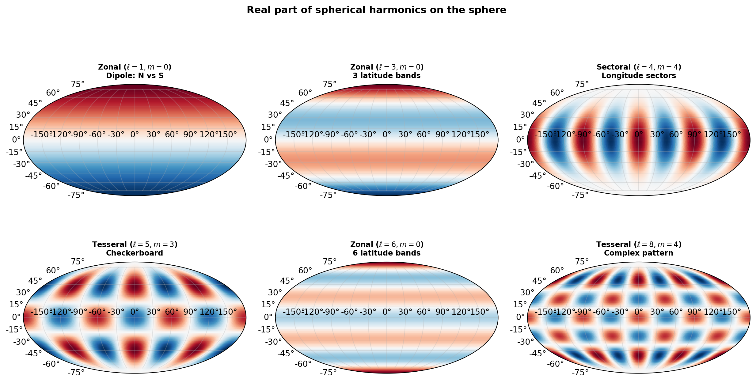
cases = [
    (1, 0, 'Zonal ($\\ell=1, m=0$)\nDipole: N vs S'),
    (3, 0, 'Zonal ($\\ell=3, m=0$)\n3 latitude bands'),
    (4, 4, 'Sectoral ($\\ell=4, m=4$)\nLongitude sectors'),
    (5, 3, 'Tesseral ($\\ell=5, m=3$)\nCheckerboard'),
    (6, 0, 'Zonal ($\\ell=6, m=0$)\n6 latitude bands'),
    (8, 4, 'Tesseral ($\\ell=8, m=4$)\nComplex pattern'),
]

fig, axes = plt.subplots(2, 3, figsize=(13, 7),
                         subplot_kw={'projection': 'mollweide'})
axes = axes.ravel()

for ax, (ell, m, title) in zip(axes, cases):
    Y = sph_harm(m, ell, PHI, THETA).real
    lon_rad = np.radians(lon - 180)
    lat_rad = np.radians(lat)
    vmax = np.abs(Y).max()
    ax.pcolormesh(lon_rad, lat_rad, Y,
                  cmap='RdBu_r', vmin=-vmax, vmax=vmax, shading='auto')
    ax.set_title(title, fontsize=9, fontweight='bold', pad=8)
    ax.grid(True, alpha=0.3)

plt.suptitle('Real part of spherical harmonics on the sphere',
             fontsize=12, fontweight='bold', y=1.02)
plt.tight_layout()
plt.show()

Part IV: Spherical Harmonics

The Full Definition

Combining the latitude and longitude parts, the spherical harmonics are:

\[\boxed{Y_\ell^m(\theta, \phi) = N_\ell^m \, P_\ell^m(\cos\theta) \, e^{im\phi}}\]

where the normalization constant is:

\[N_\ell^m = \sqrt{\frac{2\ell+1}{4\pi} \cdot \frac{(\ell-m)!}{(\ell+m)!}}\]

This normalization ensures orthonormality on the unit sphere:

\[\int_0^{2\pi}\!\int_0^{\pi} Y_\ell^m(\theta,\phi) \, Y_{\ell'}^{m'*}(\theta,\phi) \,\sin\theta\, d\theta\, d\phi = \delta_{\ell\ell'} \delta_{mm'}\]

The \(^*\) denotes complex conjugation. The \(\sin\theta\) is the Jacobian of spherical coordinates — it accounts for the fact that cells near the poles are smaller.

Important

Convention warning: Different fields use different sign conventions and normalizations. Geophysics often uses the Schmidt semi-normalized harmonics. Quantum mechanics uses the convention shown here (with the Condon–Shortley phase \((-1)^m\)). Always check which convention your software uses.

Anatomy of \(Y_\ell^m\)

Let’s unpack the pieces one more time:

\[Y_\ell^m(\theta, \phi) = \underbrace{N_\ell^m}_{\text{normalization}} \cdot \underbrace{P_\ell^m(\cos\theta)}_{\text{latitude structure}} \cdot \underbrace{e^{im\phi}}_{\text{longitude structure}}\]

The latitude part \(P_\ell^m(\cos\theta)\):

• Real-valued
• Has \(\ell - |m|\) zeros between the poles
• Near the poles: behaves like \((\sin\theta)^{|m|}\)
• For \(m=0\): reduces to ordinary Legendre \(P_\ell\)

The longitude part \(e^{im\phi}\):

• Complex-valued
• \(e^{im\phi} = \cos(m\phi) + i\sin(m\phi)\)
• Real part → \(\cos(m\phi)\): peaks at \(\phi = 0\)
• Imaginary part → \(\sin(m\phi)\): peaks at \(\phi = \pi/(2m)\)
• Together they encode amplitude and longitudinal position

Tip

The real and imaginary parts are just cosine and sine — a phase-shifted pair. A coefficient with large real part and small imaginary part places a feature near \(\phi = 0\). Equal real and imaginary parts place it at \(\phi = \pi/(4m)\). The magnitude \(|a_\ell^m|\) gives the amplitude; \(\arg(a_\ell^m)\) gives the longitudinal position.

The Complex Coefficients: Amplitude and Phase

For a single mode \((l, m)\) with coefficient \(a_\ell^m = |a_\ell^m| e^{i\alpha}\):

\[a_\ell^m \, e^{im\phi} = |a_\ell^m| \, e^{i(m\phi + \alpha)}\]

Expanding into real and imaginary parts:

\[= |a_\ell^m| \left[\cos(m\phi + \alpha) + i\sin(m\phi + \alpha)\right]\]

The physical field (which is real) uses either the real part, or equivalently, sums over \(\pm m\):

\[a_\ell^m Y_\ell^m + a_\ell^{-m} Y_\ell^{-m} \propto |a_\ell^m| \cos(m\phi + \alpha) \cdot P_\ell^{|m|}(\cos\theta)\]

Key insight: The phase \(\alpha = \arg(a_\ell^m) = \text{atan2}(\text{Im}(a_\ell^m), \text{Re}(a_\ell^m))\) controls where in longitude the pattern sits.

• Rotating the entire field eastward by \(\Delta\phi\) just multiplies: \(a_\ell^m \to a_\ell^m \, e^{im\Delta\phi}\)
• The magnitude \(|a_\ell^m|\) is unchanged — rotation is a pure phase shift in spectral space

import numpy as np
import matplotlib.pyplot as plt

phi = np.linspace(0, 2 * np.pi, 500)
m = 3

fig, axes = plt.subplots(1, 3, figsize=(12, 3))

phases = [0, np.pi / 6, np.pi / 3]
labels = [r'$\alpha = 0$', r'$\alpha = \pi/6$', r'$\alpha = \pi/3$']
colors = ['steelblue', 'tomato', 'seagreen']

for ax, alpha, label, color in zip(axes, phases, labels, colors):
    signal = np.cos(m * phi + alpha)
    ax.plot(np.degrees(phi), signal, color=color, linewidth=2)
    ax.axhline(0, color='k', linewidth=0.5)
    ax.set_xlabel(r'Longitude $\phi$ (°)')
    ax.set_ylabel(r'$\cos(m\phi + \alpha)$')
    ax.set_title(f'm={m}, {label}', fontweight='bold')
    ax.set_xlim(0, 360)
    ax.grid(True, alpha=0.3)
    # Mark the peak
    peak_phi = -alpha / m
    if peak_phi < 0:
        peak_phi += 2 * np.pi / m
    ax.axvline(np.degrees(peak_phi), color=color, linestyle='--', alpha=0.7)
    ax.text(np.degrees(peak_phi) + 5, 0.8, 'peak', fontsize=8, color=color)

plt.suptitle('Phase α shifts the feature in longitude — magnitude stays the same',
             fontsize=11, style='italic', y=1.04)
plt.tight_layout()
plt.show()

Spectral Expansion of a Real Field

Any square-integrable function on the sphere can be expanded as:

\[f(\theta, \phi) = \sum_{\ell=0}^{\infty} \sum_{m=-\ell}^{\ell} a_\ell^m \, Y_\ell^m(\theta, \phi)\]

The coefficients are obtained by projection (using orthonormality):

\[a_\ell^m = \int_0^{2\pi}\!\int_0^{\pi} f(\theta, \phi) \, Y_\ell^{m*}(\theta, \phi) \, \sin\theta \, d\theta \, d\phi\]

For real-valued fields \(f(\theta,\phi) \in \mathbb{R}\), the coefficients satisfy the conjugate symmetry:

\[a_\ell^{-m} = (-1)^m \, (a_\ell^m)^*\]

This means negative-\(m\) coefficients are redundant — we only need to store \(m \geq 0\). This is exactly analogous to the Hermitian symmetry of the Fourier transform of a real signal.

Practical storage: A truncation at degree \(\ell_{\max}\) has:

\[\sum_{\ell=0}^{\ell_{\max}} (2\ell + 1) = (\ell_{\max} + 1)^2 \quad\text{total coefficients}\]

but only \(\sum_{\ell=0}^{\ell_{\max}} (\ell + 1) = \frac{(\ell_{\max}+1)(\ell_{\max}+2)}{2}\) independent complex coefficients (for \(m \geq 0\)).

The Triangle of Spectral Coefficients

The coefficients \(a_\ell^m\) live on a triangular grid in \((\ell, m)\) space:

import numpy as np
import matplotlib.pyplot as plt

lmax = 8

fig, ax = plt.subplots(figsize=(8, 5))

for ell in range(lmax + 1):
    for m in range(-ell, ell + 1):
        if m == 0:
            color = 'tomato'
            marker = 's'
            label = 'Zonal (m=0), real' if ell == 0 else None
        elif m > 0:
            color = 'steelblue'
            marker = 'o'
            label = 'Stored (m>0), complex' if ell == 1 and m == 1 else None
        else:
            color = 'lightgray'
            marker = 'x'
            label = 'Redundant (m<0), derived from m>0' if ell == 1 and m == -1 else None
        ax.plot(m, ell, marker=marker, color=color, markersize=8, markeredgewidth=1.5)
        if label:
            ax.plot([], [], marker=marker, color=color, markersize=8,
                    linestyle='none', label=label)

ax.set_xlabel('Order $m$', fontsize=12)
ax.set_ylabel('Degree $\\ell$', fontsize=12)
ax.set_title('Spectral coefficient triangle', fontsize=13, fontweight='bold')
ax.set_xlim(-lmax - 1, lmax + 1)
ax.set_ylim(-0.5, lmax + 0.5)
ax.invert_yaxis()
ax.legend(fontsize=9, loc='lower right')
ax.grid(True, alpha=0.2)
ax.set_aspect('equal')
plt.tight_layout()
plt.show()

Note

Reading this triangle:

• Each row is a fixed degree \(\ell\) (fixed spatial scale).
• Within a row, moving to higher \(|m|\) shifts structure from latitudinal to longitudinal.
• \(m=0\) coefficients (red squares) are always real for a real field — they describe the zonal mean at each scale.
• \(m>0\) coefficients are complex — their magnitude and phase encode how much longitudinal structure exists and where it’s positioned.

Part V: The Power Spectrum

Power Per Degree: The Angular Power Spectrum

The angular power spectrum sums the energy across all orders at each degree:

\[C_\ell = \frac{1}{2\ell+1} \sum_{m=-\ell}^{\ell} |a_\ell^m|^2\]

This tells you how much variance is at each spatial scale, regardless of orientation.

• \(C_0\): the global mean squared
• \(C_1\): the dipole (hemispheric contrast) — e.g. land/ocean distribution
• Low \(\ell\): large-scale patterns (planetary waves)
• High \(\ell\): small-scale features (storms, fronts)

Parseval’s theorem on the sphere:

\[\int |f(\theta,\phi)|^2 \, d\Omega = \sum_{\ell=0}^{\infty} \sum_{m=-\ell}^{\ell} |a_\ell^m|^2 = \sum_\ell (2\ell+1) C_\ell\]

Total variance = sum of spectral power at all scales. No energy is lost or created by the transform.

Example: Power Spectra of Geophysical Fields

import numpy as np
import matplotlib.pyplot as plt
from scipy.special import sph_harm

# Synthesize two fields: smooth temperature vs sharp vorticity-like
rng = np.random.default_rng(42)
lmax = 50

# Smooth field: power ∝ ell^(-3) (like temperature)
C_smooth = np.array([(ell + 1)**(-3) for ell in range(lmax + 1)])

# Sharp field: power ∝ ell^(-1) (like vorticity / enstrophy cascade)
C_sharp = np.array([(ell + 1)**(-1) for ell in range(lmax + 1)])

fig, ax = plt.subplots(figsize=(8, 4.5))
ell_vals = np.arange(lmax + 1)

ax.loglog(ell_vals[1:], C_smooth[1:], 'o-', color='steelblue',
          markersize=3, linewidth=1.5, label=r'Smooth field: $C_\ell \propto \ell^{-3}$ (e.g. temperature)')
ax.loglog(ell_vals[1:], C_sharp[1:], 's-', color='tomato',
          markersize=3, linewidth=1.5, label=r'Sharp field: $C_\ell \propto \ell^{-1}$ (e.g. vorticity)')

# Truncation line
ell_trunc = 21
ax.axvline(ell_trunc, color='gray', linestyle='--', linewidth=1.5, alpha=0.7)
ax.text(ell_trunc + 1, 1e-1, f'T{ell_trunc} truncation', fontsize=9, color='gray')

ax.set_xlabel(r'Degree $\ell$', fontsize=12)
ax.set_ylabel(r'Power $C_\ell$', fontsize=12)
ax.set_title('Angular power spectra: smooth vs. sharp fields', fontweight='bold')
ax.legend(fontsize=9)
ax.grid(True, alpha=0.3, which='both')
plt.tight_layout()
plt.show()

The ML Connection

Notice the vorticity-like field has significant power at high \(\ell\). Truncating at \(T21\) (vertical dashed line) cuts off far more of the sharp field’s variance than the smooth field’s. This is why an ML emulator using truncated spherical harmonics can capture temperature well but fail on vorticity — the important information lives above the truncation.

This is exactly the Galewsky problem: the instability cascades energy to high \(\ell\), but a truncated spectral model can’t represent it.

Part VI: Truncation, Gibbs, and the Limits of Spectral Representations

Truncation: Cutting Off the Series

In practice we truncate the expansion at some maximum degree \(\ell_{\max}\):

\[f(\theta,\phi) \approx \sum_{\ell=0}^{\ell_{\max}} \sum_{m=-\ell}^{\ell} a_\ell^m \, Y_\ell^m(\theta,\phi)\]

This is called a T\(\ell_{\max}\) truncation. Common choices:

Truncation	Approx. resolution	Typical use
T21	~600 km	Toy models, ML prototypes
T42	~300 km	Coarse climate models
T85	~150 km	Standard climate
T170	~75 km	High-resolution climate
T639	~20 km	Operational weather (ECMWF)
T1279	~10 km	High-res weather

What happens to features smaller than the truncation scale?

They are either aliased (if your grid is too coarse to sample them) or simply absent. For smooth fields, the truncated series converges rapidly. For sharp features… it doesn’t.

The Gibbs Phenomenon on the Sphere

Just like Fourier series overshoot near a discontinuity, truncated spherical harmonic expansions produce ringing artifacts near sharp gradients.

import numpy as np
import matplotlib.pyplot as plt
from scipy.special import legendre

# 1D demo: step function expanded in Legendre polynomials
x = np.linspace(-1, 1, 2000)

# Step function: 1 for x > 0 (Northern Hemisphere), 0 for x < 0
f_true = np.where(x > 0, 1.0, 0.0)

fig, ax = plt.subplots(figsize=(9, 4.5))
ax.plot(x, f_true, 'k--', linewidth=2, label='True (step)', alpha=0.5)

for lmax, color in [(5, '#b3cde3'), (15, '#6baed6'), (40, '#2171b5'), (100, '#08306b')]:
    f_approx = np.zeros_like(x)
    for ell in range(lmax + 1):
        Pl = legendre(ell)
        # Coefficient: (2l+1)/2 * integral of f * P_l
        coeff = (2 * ell + 1) / 2 * np.trapz(f_true * Pl(x), x)
        f_approx += coeff * Pl(x)
    ax.plot(x, f_approx, color=color, linewidth=1.5,
            label=f'T{lmax} ({lmax+1} terms)')

ax.set_xlabel(r'$x = \cos\theta$', fontsize=11)
ax.set_ylabel('$f(x)$', fontsize=11)
ax.set_title('Gibbs phenomenon: Legendre expansion of a step function',
             fontweight='bold')
ax.legend(fontsize=9)
ax.set_ylim(-0.2, 1.3)
ax.grid(True, alpha=0.3)
plt.tight_layout()
plt.show()

The ~9% Overshoot Never Goes Away

No matter how many terms you add, the overshoot near the discontinuity converges to about 9% of the jump (the Gibbs constant: \(\frac{1}{\pi}\int_0^\pi \frac{\sin t}{t}dt - \frac{1}{2} \approx 0.0895\)). Higher truncation makes the ringing narrower but not smaller. This is a fundamental limitation of representing sharp features with smooth global basis functions.

This is why your ML emulator cannot learn sharp gradients in spectral space — the representation itself is incapable of capturing them cleanly.

Why This Kills ML Emulators for Sharp Features

The training problem:

1. Target field has a sharp front
2. In spectral space, this front requires precise phase coherence across \(O(\ell_{\max})\) coefficients
3. The loss landscape for getting all those phases right simultaneously is extremely rugged
4. The network learns the magnitudes (power spectrum) easily — low-frequency first (spectral bias / F-principle)
5. The phases remain noisy → the reconstruction is smeared

The representation problem:

1. Even a perfect spectral fit produces Gibbs ringing
2. The ringing is not physical — so the model is learning to approximate something that’s already a distorted version of the truth
3. The loss function penalizes ringing artifacts equally with physical errors
4. The model may learn to suppress ringing by over-smoothing — which kills the front entirely

The Way Forward

This is why hybrid architectures make sense:

• Use spectral components for what they’re good at: smooth, large-scale, balanced flow
• Use local operators (DISCO convolutions, graph neural networks) for sharp, localized features
• Let the model learn the decomposition between the two

Part VII: Spectral Transforms in Practice

The Spherical Harmonic Transform (SHT)

The forward transform (grid → spectral):

\[a_\ell^m = \int_0^{2\pi}\!\int_0^{\pi} f(\theta,\phi) \, Y_\ell^{m*}(\theta,\phi) \, \sin\theta \, d\theta \, d\phi\]

is computed in two steps:

Step 1: FFT in longitude (for each latitude ring)

\[\hat{f}_m(\theta) = \frac{1}{2\pi}\int_0^{2\pi} f(\theta,\phi) \, e^{-im\phi} \, d\phi\]

This is just a standard FFT — fast, \(O(N \log N)\) per latitude ring.

Step 2: Legendre transform in latitude

\[a_\ell^m = \int_0^{\pi} \hat{f}_m(\theta) \, \bar{P}_\ell^m(\cos\theta) \, \sin\theta \, d\theta\]

where \(\bar{P}_\ell^m\) is the normalized associated Legendre function. This integral is computed using Gaussian quadrature on a set of carefully chosen latitude points (Gauss–Legendre nodes).

Note

The inverse transform reverses the order: Legendre synthesis per \(m\), then inverse FFT. This is how spectral weather models operate at every timestep: transform to spectral space, compute linear terms, transform back, compute nonlinear terms on the grid.

Transform–Grid–Transform: How Spectral Models Work

Modern spectral models (e.g., ECMWF’s IFS) use the transform method:

┌─────────────────────────────────────────────────────────┐
│                    One timestep                          │
│                                                          │
│  Spectral space              Grid (physical) space       │
│  ─────────────              ───────────────────────      │
│  • Linear terms             • Nonlinear terms            │
│    (diffusion,                (advection u·∇f,           │
│     Coriolis)                  products, physics)        │
│                                                          │
│        ──── inverse SHT ──→                              │
│        ←─── forward SHT ───                              │
│                                                          │
│  Why? Derivatives are       Why? Products of fields      │
│  trivial in spectral        are trivial on the grid      │
│  space (multiply by ℓ)      (pointwise multiply)         │
└─────────────────────────────────────────────────────────┘

Derivatives in spectral space are algebraic, not numerical:

The Laplacian of a spherical harmonic is:

\[\nabla^2_S Y_\ell^m = -\frac{\ell(\ell+1)}{R^2} Y_\ell^m\]

So \(\nabla^2 f\) in spectral space is just: multiply \(a_\ell^m\) by \(-\ell(\ell+1)/R^2\). No finite-difference stencils, no numerical dispersion, no grid imprinting. This is the main advantage of spectral methods.

A Minimal Python Example

import numpy as np
from scipy.special import sph_harm
import matplotlib.pyplot as plt

# Create a simple field and do forward/inverse SHT manually (low resolution)
lmax = 20
ntheta = 2 * lmax + 2  # Gauss-Legendre quadrature needs >= lmax+1 points
nphi = 2 * (2 * lmax + 1)

# Gauss-Legendre quadrature points and weights
x_gl, w_gl = np.polynomial.legendre.leggauss(ntheta)
theta_gl = np.arccos(x_gl)
phi_gl = np.linspace(0, 2 * np.pi, nphi, endpoint=False)
THETA, PHI = np.meshgrid(theta_gl, phi_gl, indexing='ij')

# Test field: a localized blob (hard for spectral methods!)
f = np.exp(-((THETA - np.pi / 3)**2 + (PHI - np.pi)**2) / 0.1)

# Forward SHT
# Step 1: FFT in longitude
f_hat = np.fft.fft(f, axis=1) / nphi  # shape: (ntheta, nphi)

# Step 2: Legendre transform
a_lm = np.zeros((lmax + 1, lmax + 1), dtype=complex)
for ell in range(lmax + 1):
    for m in range(ell + 1):
        # Compute normalized associated Legendre values at quadrature points
        Ylm_vals = sph_harm(m, ell, 0, theta_gl)  # Y at phi=0 → just N * P_l^m
        # Project: sum over latitude with quadrature weights
        # f_hat[:, m] is the m-th Fourier coefficient at each latitude
        a_lm[ell, m] = 2 * np.pi * np.sum(
            f_hat[:, m] * np.conj(Ylm_vals) * w_gl
        )

# Power spectrum
Cl = np.zeros(lmax + 1)
for ell in range(lmax + 1):
    power = abs(a_lm[ell, 0])**2
    for m in range(1, ell + 1):
        power += 2 * abs(a_lm[ell, m])**2  # factor 2 for negative m
    Cl[ell] = power / (2 * ell + 1)

fig, axes = plt.subplots(1, 2, figsize=(11, 4))

ax = axes[0]
lat = 90 - np.degrees(THETA)
lon = np.degrees(PHI)
c = ax.contourf(lon, lat, f, levels=20, cmap='YlOrRd')
plt.colorbar(c, ax=ax, shrink=0.8, label='f')
ax.set_xlabel('Longitude (°)')
ax.set_ylabel('Latitude (°)')
ax.set_title('Original field (localized blob)', fontweight='bold')

ax = axes[1]
ax.semilogy(range(1, lmax + 1), Cl[1:], 'o-', color='steelblue', markersize=4)
ax.set_xlabel(r'Degree $\ell$')
ax.set_ylabel(r'Power $C_\ell$')
ax.set_title('Angular power spectrum', fontweight='bold')
ax.grid(True, alpha=0.3)

plt.tight_layout()
plt.show()

Note

Notice how the localized blob spreads its energy across all degrees — a localized feature has a broad spectrum. This is the uncertainty principle on the sphere: spatial localization requires spectral delocalization, and vice versa. This is the fundamental tension when using spherical harmonics for ML.

Part VIII: Summary and Connections

The Complete Picture

Building blocks:

Component	Role
\(e^{im\phi}\)	Longitude structure (Fourier)
\(P_\ell^m(\cos\theta)\)	Latitude structure (Legendre)
\(Y_\ell^m = N P_\ell^m e^{im\phi}\)	Full basis function on sphere
\(a_\ell^m\)	Complex coefficient = amplitude + phase
\(\ell\)	Degree → total spatial scale
\(m\)	Order → longitudinal wavenumber

Key properties:

Property	Why it matters
Orthonormality	Clean decomposition, Parseval holds
Eigenfunctions of \(\nabla^2_S\)	Derivatives become multiplication
Global support	Great for smooth fields
Global support	Terrible for sharp local features
Conjugate symmetry	Real fields → only store \(m \geq 0\)
Truncation → Gibbs	Fundamental limit on sharp features

Cheat Sheet: Reading Spectral Coefficients

Given coefficients \(a_\ell^m\), here’s what you can read off immediately:

• \(a_0^0\): proportional to the global mean of the field (\(\bar{f} = a_0^0 \sqrt{4\pi}\) for orthonormal harmonics)
• \(a_\ell^0\) (all real): the zonal mean structure at scale \(\ell\) — no longitude dependence
• \(|a_\ell^m|\) for \(m > 0\): how much wave-\(m\) longitudinal structure exists at scale \(\ell\)
• \(\arg(a_\ell^m)\) for \(m > 0\): the longitudinal position of that structure
• \(C_\ell = \frac{1}{2\ell+1}\sum_m |a_\ell^m|^2\): total variance at scale \(\ell\), regardless of direction
• Steep \(C_\ell\) decay (e.g. \(\ell^{-3}\)): smooth field, low truncation is fine
• Shallow \(C_\ell\) decay (e.g. \(\ell^{-1}\)): sharp features, high truncation needed, Gibbs will hurt

Connections to ML on the Sphere

Why spectral methods are attractive for ML:

• Exact derivatives (no discretization error)
• Natural handling of periodicity in longitude
• Built-in smoothness regularization
• Efficient global communication
• Rotation equivariance is natural

Where they struggle:

• Sharp gradients → Gibbs phenomenon
• Local features → spectral delocalization
• Phase coherence → hard optimization
• Spectral bias in NNs compounds the issue
• Nonlinear interactions → expensive convolutions in spectral space

The Design Principle

Match the inductive bias to the physics:

• Smooth, global, balanced dynamics → Spherical harmonics are the right basis
• Sharp, local, nonlinear dynamics → Local operators (DISCO, GNNs, wavelets) are better
• Both at once (which is most of geophysics) → Hybrid architectures

Key Takeaways

1. Spherical harmonics = Fourier in longitude × Legendre in latitude. They are the natural orthogonal basis for the sphere, arising from separation of variables in the Laplacian.

2. Degree \(\ell\) = spatial scale, order \(m\) = longitudinal wavenumber. Together they give \((\ell_{\max}+1)^2\) total modes up to truncation.

3. The complex exponential \(e^{im\phi}\) encodes both amplitude and position via its magnitude and phase. The real and imaginary parts are cosine and sine — a phase pair that locates features in longitude.

4. The power spectrum \(C_\ell\) tells you where the energy is across scales. Steep decay = smooth field. Shallow decay = sharp features that need high truncation.

5. Truncation produces Gibbs ringing near sharp gradients — an inherent limitation, not a bug. No amount of training will overcome a representational bottleneck.

6. For ML: spectral representations are powerful for smooth dynamics but fundamentally limited for sharp local features. This motivates hybrid architectures that combine global spectral and local spatial operators.

Recommended Reading

Textbooks:

• Durran (2010): Numerical Methods for Fluid Dynamics — Chapter 8 (spectral methods)
• Holton & Hakim (2013): An Introduction to Dynamic Meteorology — Appendix on spherical harmonics
• Jackson (1999): Classical Electrodynamics — Chapter 3 (the physics derivation)
• Arfken, Weber & Harris: Mathematical Methods for Physicists — Chapter 15 (comprehensive reference)

For the ML connection:

• Bonev et al. (2023): “Spherical Fourier Neural Operators” (SFNO) — spectral ML on the sphere
• Ocampo et al. (2022): “DISCO: Discrete-Continuous Convolutions” — local operators on the sphere
• Rahaman et al. (2019): “On the Spectral Bias of Neural Networks” — the F-principle

Software:

• scipy.special.sph_harm — evaluation of \(Y_\ell^m\)
• SHTns — fast spherical harmonic transforms (C library with Python bindings)
• torch-harmonics (NVIDIA) — GPU-accelerated SHT for ML
• healpy — HEALPix pixelization + SHT (from CMB cosmology)