ATOC 4815/5815
Numerical Integration & Explicit Euler
CU Boulder ATOC
2026-01-01
Numerical Integration
Today’s Objectives
- Understand when and why we need numerical integration
- Master the Explicit Euler method for solving ODEs
- Apply Euler method to atmospheric science problems
- Prepare for implementing Lorenz63 model (midterm!)
Reminders
Midterm Coming Soon!
- Focus: NumPy, Python fundamentals, Explicit Euler
- Practice: Lorenz63 class structure
Office Hours:
Will: Tu 11:15-12:15p Th 9-10a Aerospace Cafe
Aiden: M / W 330-430p DUAN D319
ATOC 4815/5815 Playlist

Why Numerical Integration?
Earth Science is Full of DiffEqs
Temperature evolution: \[\frac{dT}{dt} = -\alpha(T - T_{env}) + H\]
Wind acceleration: \[\frac{du}{dt} = -\frac{1}{\rho}\frac{\partial p}{\partial x} + fv\]
Lorenz63 chaotic system: \[\frac{dx}{dt} = \sigma(y - x)\] \[\frac{dy}{dt} = \rho x - y - xz\] \[\frac{dz}{dt} = xy - \beta z\]
What Does It Mean to “Solve” an DiffEq?
Say we have an initial value problem:
\[\frac{dy}{dt} = f(t, y), \quad y(t_0) = y_0\]
Goal: Find the trajectory \(y(t)\) for \(t > t_0\)
Two options:
- Analytical integration → exact equation for \(y(t)\)
- Numerical integration → approximation for \(y(t)\)
Analytical Integration: The Dream
Example: Simple exponential decay
\[\frac{dT}{dt} = -\alpha T, \quad T(0) = T_0\]
Analytical solution:
\[T(t) = T_0 e^{-\alpha t}\]
Perfect! We have an exact formula for any time \(t\).
Analytical Integration: The Reality
Lorenz63 equations:
\[\frac{dx}{dt} = \sigma(y - x)\] \[\frac{dy}{dt} = \rho x - y - xz\] \[\frac{dz}{dt} = xy - \beta z\]
No analytical solution exists! 😱
Most real-world systems do not have analytical solutions.
We need numerical methods.
Numerical Integration: The Only Option
Key insight: Most real-world systems cannot be solved analytically
Good news: Extensive research and software tools exist!
- Many methods optimized for different problems
- Industry applications drive development
- Python has excellent tools (
scipy,numpy)
Explicit Euler Method
The Big Idea
Can’t solve exactly? Approximate step by step!
Replace derivative \(\frac{dy}{dt}\) with finite difference:
\[\frac{dy}{dt} \approx \frac{y_{n+1} - y_n}{\Delta t}\]
Substitute into ODE:
\[\frac{y_{n+1} - y_n}{\Delta t} = f(t_n, y_n)\]
Explicit Euler Formula
Rearrange to solve for \(y_{n+1}\):
\[y_{n+1} = y_n + f(t_n, y_n) \cdot \Delta t\]
Where:
- \(y_n\) = state at current time step \(n\)
- \(y_{n+1}\) = state at next time step \(n+1\)
- \(f(t_n, y_n)\) = tendency (rate of change)
- \(\Delta t\) = time step size
Visual Interpretation: Forward Euler
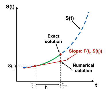
Key idea: Use the slope \(F(t_i, S(t_i))\) at the current point to step forward
- Exact solution: True trajectory (blue curve)
- Numerical solution: Approximate trajectory using tangent line (red segments)
- Error accumulates: Each step introduces small error
Simple Example: Exponential Decay
\[\frac{dT}{dt} = -0.5T, \quad T(0) = 100, \quad \Delta t = 0.1\]
Step 1: \[T_1 = T_0 + f(t_0, T_0) \cdot \Delta t = 100 + (-0.5 \times 100) \times 0.1 = 95\]
Step 2: \[T_2 = T_1 + f(t_1, T_1) \cdot \Delta t = 95 + (-0.5 \times 95) \times 0.1 = 90.25\]
Step 3: \[T_3 = T_2 + f(t_2, T_2) \cdot \Delta t = 90.25 + (-0.5 \times 90.25) \times 0.1 \approx 85.74\]
Implementing Euler in Python
Full Integration Loop
def integrate(y0, f, dt, n_steps):
    """Integrate ODE using Explicit Euler

    Args:
        y0: initial condition
        f: tendency function
        dt: time step
        n_steps: number of time steps

    Returns:
        trajectory: array of states over time
    """
    trajectory = [y0]
    y = y0

    for step in range(n_steps):
        y = euler_step(y, f, dt)
        trajectory.append(y)

    return np.array(trajectory)
Lorenz63 with Explicit Euler
The Lorenz63 System
Edward Lorenz (1963) explored deterministic chaos with:
\[\frac{dx}{dt} = \sigma(y - x)\] \[\frac{dy}{dt} = \rho x - y - xz\] \[\frac{dz}{dt} = xy - \beta z\]
Standard parameters: \(\sigma = 10\), \(\rho = 28\), \(\beta = 8/3\)
Typical initial condition: \((x_0, y_0, z_0) = (1, 1, 1)\)
Applying Euler to Lorenz63
Step 1: Define tendency function
Applying Euler to Lorenz63 (cont.)
Step 2: Time step with Euler
That’s it! This is what you’ll implement for the midterm.
Lorenz63 Class Structure
class Lorenz63:
    def __init__(self, sigma=10, rho=28, beta=8/3, dt=0.01):
        self.sigma = sigma
        self.rho = rho
        self.beta = beta
        self.dt = dt

    def tendency(self, state):
        """Calculate derivatives"""
        x, y, z = state
        dx_dt = self.sigma * (y - x)
        dy_dt = self.rho * x - y - x * z
        dz_dt = x * y - self.beta * z
        return np.array([dx_dt, dy_dt, dz_dt])

    def step(self, state):
        """One Euler step"""
        return state + self.tendency(state) * self.dt

    def integrate(self, state0, n_steps):
        """Full integration"""
        trajectory = [state0]
        state = state0
        for _ in range(n_steps):
            state = self.step(state)
            trajectory.append(state)
        return np.array(trajectory)
Midterm Prep: Logistic Growth
The Logistic Growth Model
Midterm Problem: Population growth with carrying capacity
\[\frac{dN}{dt} = r \cdot N \cdot \left(1 - \frac{N}{K}\right)\]
Where:
- \(N\) = population at time \(t\)
- \(r\) = growth rate
- \(K\) = carrying capacity
- \(\frac{dN}{dt}\) = rate of change of population
Deriving the Time Stepping Equation
Start with Euler formula: \[N_{n+1} = N_n + f(N_n) \cdot \Delta t\]
Substitute tendency function: \[N_{n+1} = N_n + r \cdot N_n \cdot \left(1 - \frac{N_n}{K}\right) \cdot \Delta t\]
This is your time stepping equation!
Logistic Growth Class Structure
class LogisticGrowth:
    def __init__(self, r, K, dt):
        """Initialize with growth rate, carrying capacity, time step"""
        self.r = r
        self.K = K
        self.dt = dt

    def tendency(self, N):
        """Calculate dN/dt given current population"""
        return self.r * N * (1 - N / self.K)

    def step(self, N):
        """Advance population by one time step"""
        dN_dt = self.tendency(N)
        N_next = N + dN_dt * self.dt
        return N_next

    def integrate(self, N0, n_steps):
        """Evolve population over multiple time steps"""
        trajectory = [N0]
        N = N0
        for _ in range(n_steps):
            N = self.step(N)
            trajectory.append(N)
        return trajectory
Midterm Prep: Key Concepts
Understand the Euler formula: \[y_{n+1} = y_n + f(t_n, y_n) \cdot \Delta t\]
Know the method structure:
__init__()→ store parameterstendency()→ calculates \(f(y)\)step()→ applies Euler formulaintegrate()→ loops through time
Practice deriving time stepping equations
Be able to write pseudo code (logic over syntax)
Accuracy and Stability
Numerical vs Analytical Solutions
Key insight: Numerical integration is always an approximation
Accuracy depends on:
- Time step size \(\Delta t\)
- The method used (Euler is simplest, not most accurate)
- The problem being solved
- Stability of the system
Smaller \(\Delta t\) generally gives better accuracy
Time Step Size Matters
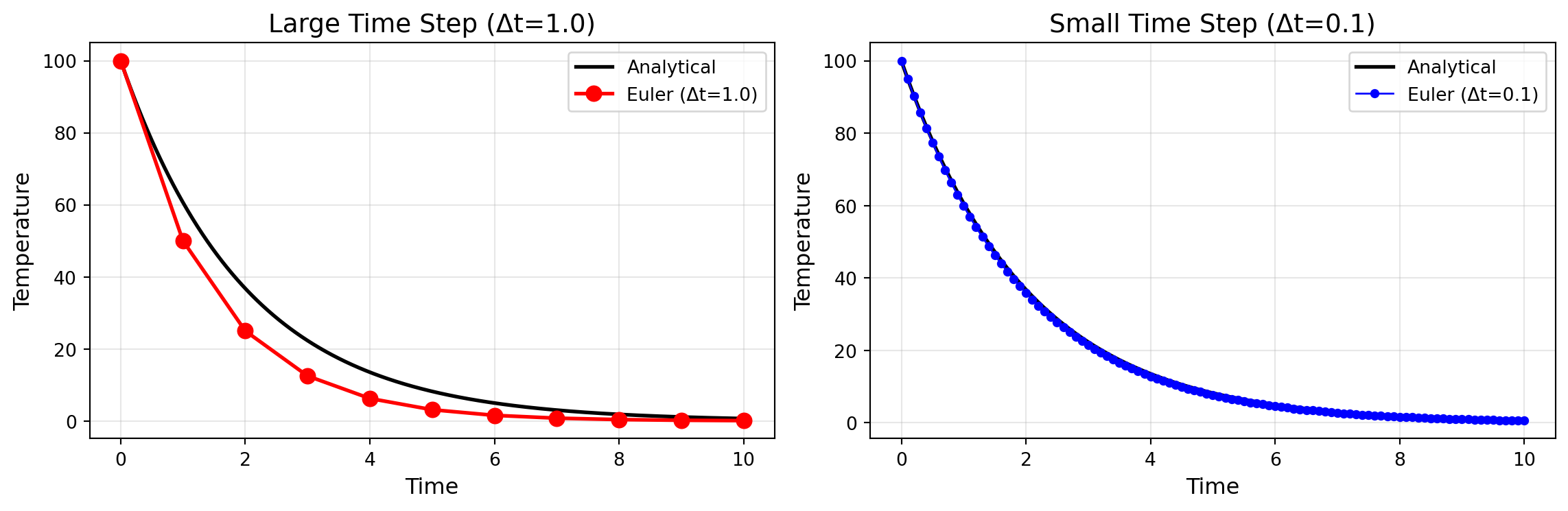
The Stability Question
Apply Euler to the linear test equation \(\;\dfrac{dy}{dt} = \lambda\, y\):
\[y_{n+1} = y_n + \Delta t\,\lambda\, y_n = \underbrace{(1 + \Delta t\,\lambda)}_{G}\; y_n\]
\(G = 1 + \Delta t\,\lambda\) is the amplification factor.
After \(n\) steps: \(\;y_n = G^n\, y_0\).
Stability criterion: \(\;|G| \le 1\)
- \(|G| < 1\): solution decays (stable)
- \(|G| = 1\): solution neither grows nor decays (neutral)
- \(|G| > 1\): solution blows up (unstable)
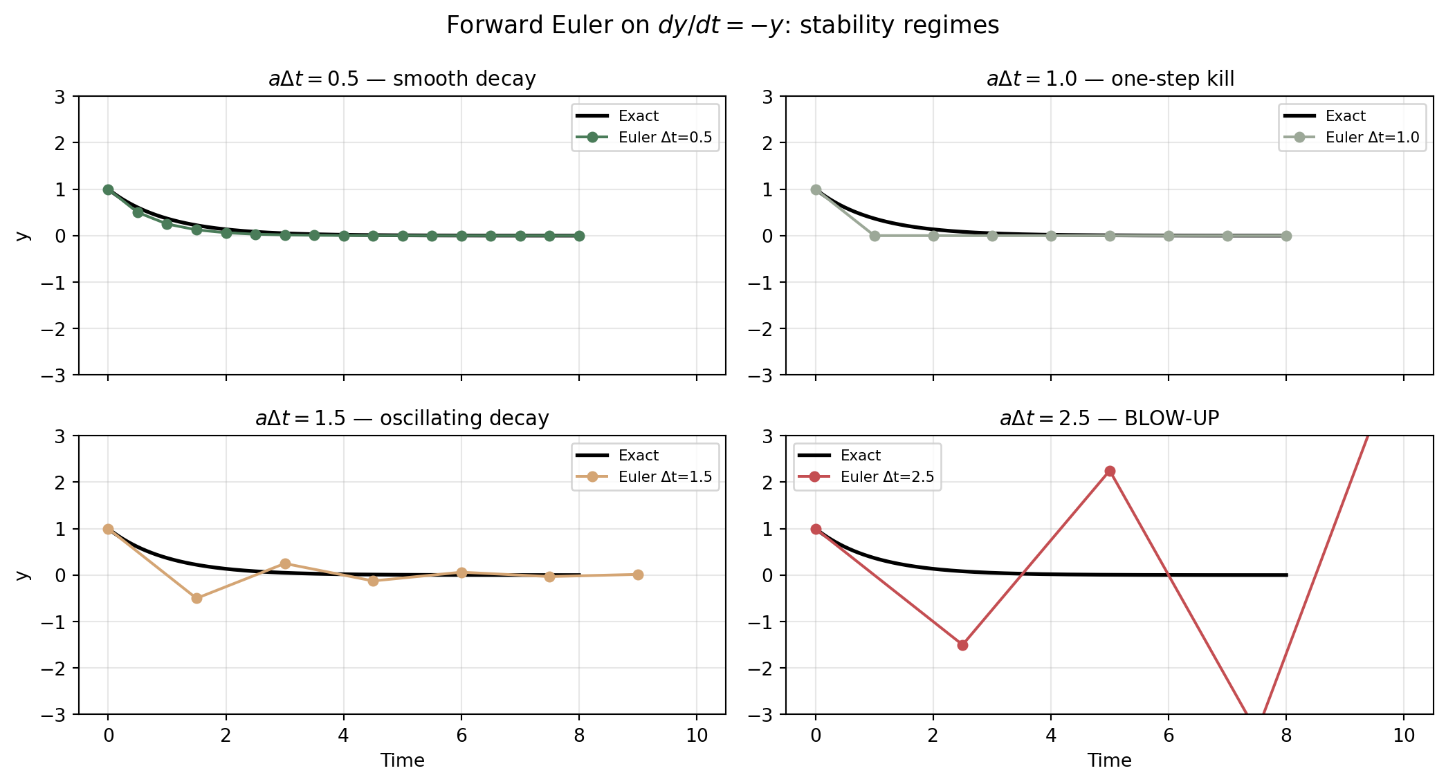
Stability for Decay (\(\lambda < 0\))
Let \(\lambda = -a\) with \(a > 0\), so \(G = 1 - a\Delta t\).
| Regime | Condition | Behavior |
|---|---|---|
| Smooth decay | \(0 < a\Delta t < 1\) | Monotone convergence to 0 |
| One-step kill | \(a\Delta t = 1\) | Jumps to 0 in one step |
| Oscillating decay | \(1 < a\Delta t < 2\) | Sign flips each step, amplitude shrinks |
| Blow-up | \(a\Delta t > 2\) | Sign flips, amplitude grows |
Stability rule for Forward Euler on decay:
\[\boxed{\Delta t < \frac{2}{a}}\]
Seeing Stability Break
The Stability Rule
For \(\;\dfrac{dy}{dt} = -a\,y\;\) (\(a > 0\)), Forward Euler is stable when:
\[\Delta t < \frac{2}{a}\]
Physical intuition: Faster dynamics (larger \(a\)) demand smaller time steps.
- \(a = 1 \;\Rightarrow\; \Delta t < 2\)
- \(a = 100 \;\Rightarrow\; \Delta t < 0.02\)
- \(a = 10^6 \;\Rightarrow\; \Delta t < 2\times10^{-6}\)
This is why weather models use small time steps!
The atmosphere contains processes with very different time scales.
When Euler Always Fails
Inertial Motion on an f-Plane
1) Setup and assumptions
We consider a parcel moving on an f-plane (constant Coriolis parameter \((f)\)) with:
- no pressure gradient force
- no friction
- horizontal velocity components \((u(t))\) (east) and \((v(t))\) (north)
So the only acceleration is due to the Coriolis force:
\[ \frac{du}{dt} = f\,v, \qquad \frac{dv}{dt} = -f\,u \]
Physical meaning: the acceleration is always perpendicular to the velocity (it turns the flow but does not speed it up).
Why the motion is perpendicular (10 seconds)
Let the horizontal velocity vector be
\[ \mathbf{u} = (u, v) \]
From the inertial (pure Coriolis) equations,
\[ \frac{d\mathbf{u}}{dt} = (f v,\,-f u) \]
Now take the dot product of velocity with its acceleration:
\[ \mathbf{u}\cdot\frac{d\mathbf{u}}{dt} = (u, v)\cdot(fv, -fu) = u(fv) + v(-fu) = fuv - fuv = 0 \]
Because the dot product is zero, the acceleration is always perpendicular to the velocity.
So Coriolis changes the direction of the flow, not its speed.
2. Turn the coupled system into one equation
Differentiate the first equation in time:
\[ \frac{d^2u}{dt^2} = f\,\frac{dv}{dt} \]
Now substitute \((\frac{dv}{dt} = -f\,u)\):
\[ \frac{d^2u}{dt^2} = f(-f u) = -f^2 u \]
So \((u(t))\) satisfies a simple harmonic oscillator:
\[ \frac{d^2u}{dt^2} + f^2 u = 0 \]
By the same steps, \((v(t))\) satisfies: \[ \frac{d^2v}{dt^2} + f^2 v = 0 \]
3. General sol’n (oscillation at frequency \((|f|)\))
A solution to \((\;u'' + f^2 u = 0\;)\) is:
\[ u(t) = A\cos(ft) + B\sin(ft) \]
Use \((\frac{du}{dt} = f v)\) to get \((v(t))\):
\[ \frac{du}{dt} = -Af\sin(ft) + Bf\cos(ft) = f v \]
So
\[ v(t) = -A\sin(ft) + B\cos(ft) \]
4. Apply a common initial condition
Suppose we start with purely eastward flow:
\[ u(0)=U_0,\qquad v(0)=0 \]
At \((t=0)\):
- \((u(0)=A = U_0)\)
- \((v(0)=B = 0)\)
So the solution becomes:
\[ u(t) = U_0\cos(ft), \qquad v(t) = -U_0\sin(ft) \]
This is inertial oscillation: the velocity vector rotates with angular frequency \((|f|)\).
The inertial period is: \[ T = \frac{2\pi}{|f|} \]
5. Key property: speed is conserved
Compute the speed:
\[ u^2 + v^2 = U_0^2\cos^2(ft) + U_0^2\sin^2(ft) = U_0^2 \]
So
\[ \sqrt{u^2 + v^2} = U_0 = \text{constant} \]
Interpretation: Coriolis changes the direction of motion but not the magnitude (no energy input or loss).
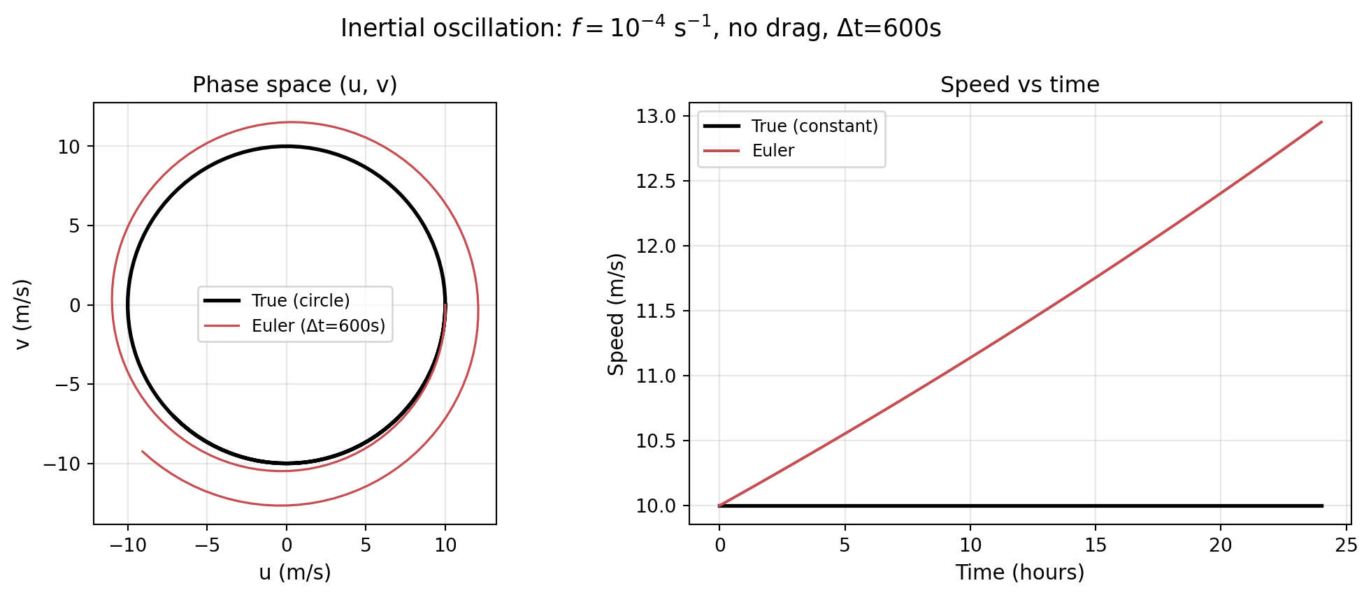
Why Euler Fails: Tangent Steps
Each Euler step follows the tangent to the circle — and lands outside it.
Proof: After one step with \(h = \Delta t\):
\[u_{n+1} = u_n + h f v_n, \qquad v_{n+1} = v_n - h f u_n\]
Compute the new radius squared:
\[R_{n+1}^2 = u_{n+1}^2 + v_{n+1}^2 = (1 + h^2 f^2)\, R_n^2\]
Since \(h^2 f^2 > 0\), the radius always grows:
\[\boxed{R_{n+1} = \sqrt{1 + h^2 f^2}\; R_n > R_n}\]
Forward Euler is unconditionally unstable for pure oscillations.
Euler Spirals Out
:::
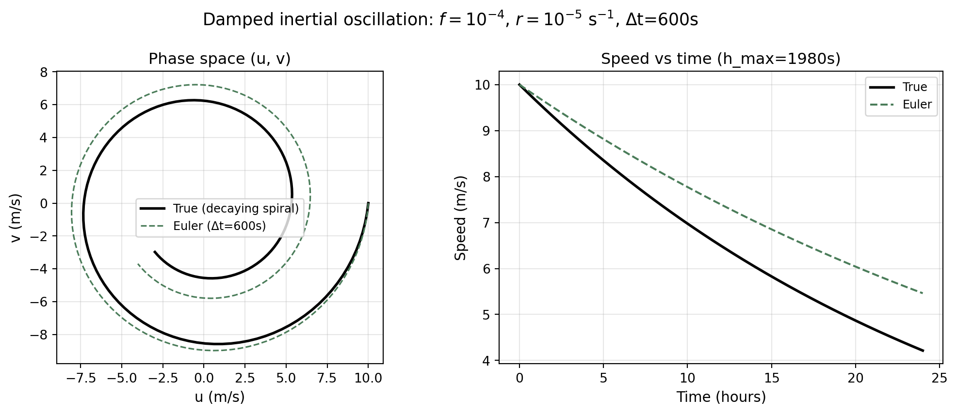
The Fix: Add Drag (Euler Form)
We add linear drag (Rayleigh friction) and integrate with Forward Euler.
Continuous equations: \[ \frac{du}{dt} = f\,v - r\,u, \qquad \frac{dv}{dt} = -f\,u - r\,v \]
1. Forward Euler update
With time step \(h\), Euler says \(N_{n+1} = N_n + h \bullet (tendency)\):
\[ u_{n+1} = u_n + h\,(f v_n - r u_n), \qquad v_{n+1} = v_n + h\,(-f u_n - r v_n) \]
Rewrite to highlight the two effects:
\[ u_{n+1} = (1-rh)\,u_n + (fh)\,v_n, \qquad v_{n+1} = -(fh)\,u_n + (1-rh)\,v_n \]
2) What happens to the radius (speed)?
Define the squared speed (“radius squared”): \[ R_n = u_n^2 + v_n^2 \]
Start from the Euler updates (drag + Coriolis): \[ u_{n+1} = (1-rh)\,u_n + (fh)\,v_n, \qquad v_{n+1} = -(fh)\,u_n + (1-rh)\,v_n \]
Compute the next-step radius: \[ R_{n+1} = u_{n+1}^2 + v_{n+1}^2 \]
Substitute: \[ R_{n+1} = \big[(1-rh)u_n + (fh)v_n\big]^2 + \big[-(fh)u_n + (1-rh)v_n\big]^2 \]
Expand each square: \[ \big[(1-rh)u_n + (fh)v_n\big]^2 = (1-rh)^2u_n^2 +2(1-rh)(fh)u_nv_n +(fh)^2v_n^2 \]
\[ \big[-(fh)u_n + (1-rh)v_n\big]^2 = (fh)^2u_n^2 -2(1-rh)(fh)u_nv_n +(1-rh)^2v_n^2 \]
Add them (cross terms cancel): \[ R_{n+1} = \Big[(1-rh)^2u_n^2+(fh)^2v_n^2\Big] + \Big[(fh)^2u_n^2+(1-rh)^2v_n^2\Big] \]
Factor: \[ R_{n+1} = \Big[(1-rh)^2+(fh)^2\Big]\,(u_n^2+v_n^2) \]
So: \[ \boxed{ R_{n+1} = \Big[(1-rh)^2+(fh)^2\Big]\,R_n } \]
3. Drag can prevent radius growth
For “no expansion” we want \(R_{n+1}\le R_n\), i.e. \(M\le 1\):
\[ (1-rh)^2 + (fh)^2 \le 1 \]
This simplifies to the step-size condition:
\[ -2rh + (r^2+f^2)h^2 \le 0 \quad\Rightarrow\quad \boxed{ h \le \frac{2r}{r^2+f^2} } \]
Interpretation: Euler tends to pump energy into inertial motion; drag removes energy. With small enough \(h\) (or large enough \(r\)), the discrete radius stops growing.
Damped Oscillation!
The Big Picture
| System | Eigenvalue \(\lambda\) | Euler Stability | Condition |
|---|---|---|---|
| Pure decay: \(y'=-ay\) | \(\lambda = -a\) (real, negative) | Conditionally stable | \(\Delta t < 2/a\) |
| Pure oscillation: \(y'=\pm ify\) | \(\lambda = \pm if\) (imaginary) | Never stable | No \(\Delta t\) works |
| Damped oscillation | \(\lambda = -r \pm if\) | Conditionally stable | \(\Delta t \le 2r/(r^2+f^2)\) |
Takeaway for real models:
- Pure oscillatory modes (gravity waves, inertial oscillations) are poison for Forward Euler
- Dissipation (friction, diffusion) can stabilize — but only if \(\Delta t\) is small enough
- This is why weather/climate models use implicit or semi-implicit methods for fast oscillations
Method vs Solver
Method: The mathematical formula/equation
- Example: Explicit Euler, Runge-Kutta, Adams-Bashforth
- Defines how to approximate \(y(t)\)
Solver: The software implementation
- Examples:
scipy.integrate.solve_ivp, Juliasolve(), our Lorenz63 class - Includes: method choice, error control, interpolation, output settings
For this course: We’re building our own solver using Explicit Euler!
Practical Tips
Debugging Your Implementation
- Start simple: Test with exponential decay first
- Check dimensions: Make sure arrays have correct shapes
- Verify tendency: Print out \(f(y)\) for known initial conditions
- Compare step sizes: Try \(\Delta t = 0.01, 0.001\) and compare
- Visualize: Plot your results - does it look reasonable?
Common Mistakes
Mistake 1: Forgetting to multiply by \(\Delta t\)
Common Mistakes (cont.)
Summary
Key Takeaways
Most diffEQs don’t have analytical solutions
- Numerical integration is essential
Explicit Euler is the simplest method: \[y_{n+1} = y_n + f(t_n, y_n) \cdot \Delta t\]
Class structure for ODE solvers:
tendency()→ rate of changestep()→ one time step forwardintegrate()→ full trajectory
Apply same pattern to any ODE system
- Logistic Growth (midterm)
- Lorenz63 (midterm bonus)
Midterm Checklist
What you need to master:
- ✓ Derive Euler time stepping from ODE equation
- ✓ Write pseudo code for LogisticGrowth class
- ✓ Understand all four class methods (
__init__,tendency,step,integrate) - ✓ Know Lorenz63 structure (bonus: calculate by hand)
- ✓ Review NumPy operations (Part 1 of exam)
- ✓ Review Python fundamentals (Part 2 of exam)
Study Resources
Practice materials:
- Simple exponential decay implementation
- Review Lorenz63 class from lecture notes
Get help:
- Office hours: Will (Tu/Th 11:15-12:15p), Aiden (M/W 3:30-4:30p)
- Practice writing pseudo code
- Test your understanding by explaining to a classmate
Questions?
Final tips:
- Focus on understanding, not memorization
- Practice the class structure pattern
- Start with simple examples, build up complexity
- Draw diagrams to visualize time stepping
You’ve got this! The concepts are straightforward once you see the pattern.
Acknowledgments
Course materials adapted from:
Fiona Majeau, ECEN 5447: Power System Dynamics, CU Boulder
Thank you for the excellent numerical integration materials!

ATOC 4815/5815 - Numerical Integration | Adapted from Fiona Majeau (ECEN 5447)