ATOC 4815: Python & Data Analysis

Demo Lecture - Introduction to Scientific Computing

Will Chapman

CU Boulder ATOC

2026-01-01

Welcome

Course Overview

  • Python programming for atmospheric science
  • Data analysis with real datasets
  • Visualization techniques
  • Final project: Independent analysis

Python Basics

Working with NumPy

Arrays are fundamental to scientific computing:

import numpy as np

# Create a temperature array (°C)
temps = np.array([15.2, 18.7, 22.1, 19.8, 16.5])

print(f"Mean temperature: {temps.mean():.1f}°C")
Mean temperature: 18.5°C

Key point: NumPy operations are vectorized and fast!

Data Structures

Lists

temps = [15, 18, 22]
temps.append(20)

✅ Flexible ❌ Slower for math

Arrays

temps = np.array([15, 18, 22])
temps_k = temps + 273.15

✅ Fast vectorized ops ✅ Built for science

Data Analysis

Loading Climate Data

Example: Working with NCEP/NCAR Reanalysis

import xarray as xr

# Open dataset
ds = xr.open_dataset('reanalysis.nc')

# Select region and time
data = ds.sel(
    lat=slice(25, 50),
    lon=slice(-125, -65),
    time='2023-01'
)

Statistical Analysis

Common operations for climate data:

  1. Time averaging: data.mean(dim='time')
  2. Spatial patterns: data.groupby('season').mean()
  3. Anomalies: data - data.mean(dim='time')
  4. Trends: Linear regression with scipy.stats

Visualization

Matplotlib Basics

import matplotlib.pyplot as plt
import numpy as np

# Generate sample data
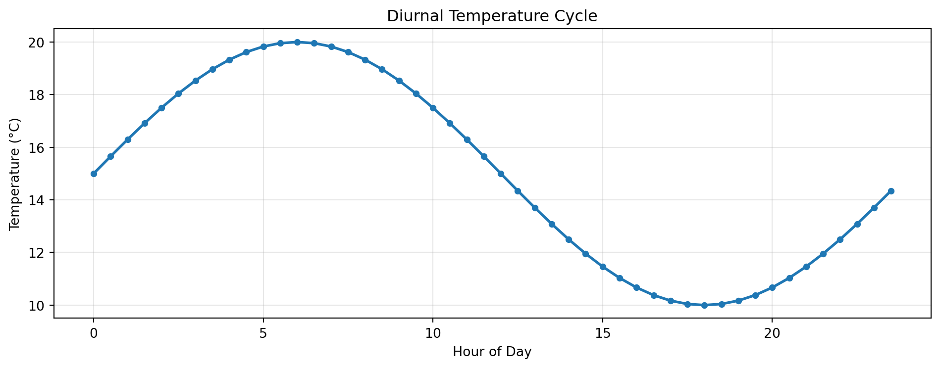
time = np.arange(0, 24, 0.5)
temp = 15 + 5 * np.sin(2 * np.pi * time / 24)

# Create plot
plt.figure(figsize=(10, 4))
plt.plot(time, temp, 'o-', linewidth=2, markersize=4)
plt.xlabel('Hour of Day')
plt.ylabel('Temperature (°C)')
plt.title('Diurnal Temperature Cycle')
plt.grid(True, alpha=0.3)
plt.tight_layout()
plt.show()

Best Practices

Good Plot ✅

  • Clear labels
  • Readable fonts
  • Appropriate colors
  • Legend when needed
  • Proper units

Avoid ❌

  • Tiny text
  • Rainbow colormap (usually)
  • 3D when 2D works
  • Chart junk
  • Missing labels

Mathematical Formulas

Atmospheric Equations

Ideal Gas Law:

\[ p = \rho R T \]

Hydrostatic Balance:

\[ \frac{\partial p}{\partial z} = -\rho g \]

Geostrophic Wind:

\[ u_g = -\frac{1}{\rho f}\frac{\partial p}{\partial y}, \quad v_g = \frac{1}{\rho f}\frac{\partial p}{\partial x} \]

Course Logistics

Weekly Structure

Day Activity
Monday Lecture & coding demo
Wednesday Lab work & debugging
Friday Discussion & code review

Grading

  • Homework (40%): Weekly coding assignments
  • Labs (30%): In-class exercises
  • Final Project (30%): Independent analysis

Resources

Getting Help

  1. Office Hours: By appointment (wchapman@colorado.edu)
  2. Course Website: willychap.github.io/course
  3. Documentation:
    • Python: docs.python.org
    • NumPy: numpy.org
    • Xarray: docs.xarray.dev
  4. Stack Overflow: For debugging

Next Week

Topics

  • File I/O
  • CSV and NetCDF
  • Data cleaning

Homework

  • Install Python environment
  • Read: Chapters 1-2
  • Complete Lab 1

Questions?

Contact

Prof. Will Chapman 📧 wchapman@colorado.edu 🌐 willychap.github.io 🏢 ATOC Building, CU Boulder

See you Wednesday!