%%{init: {'theme': 'default'}}%%
graph TD
    A["CAM6<br/>(full physics)"] -->|"train on 30 yrs"| B["CAMulator<br/>(AI emulator)"]
    D["Prescribed SST<br/>(AMIP-style)"] -->|"training regime"| B
    B -->|"350× faster"| C["Large ensembles<br/>Centennial runs"]
    E["Live POP2 SST<br/>(this work)"] -.->|"new frontier"| B
POP goes the CAMulator
Initial Results: CAMulator ↔︎ POP2 inside CESM2/3
Will Chapman | CU Boulder
The Scientific Gap
We have been working significantly with uncoupled systems:
| Mode | Atmosphere | Ocean |
|---|---|---|
| AMIP | active | prescribed SST/ICE |
| OMIP / GIAF | prescribed ATM | active |
| This work | ML ATM | active |
The problem:
- In OMIP, the ocean responds to forcing — but the forcing never changes based on what the ocean does
- Warm SST anomalies can’t generate more evaporation, shift the jet stream, or modify precipitation
- Interactive air-sea feedback is missing
Why it matters:
- The climate system is coupled
- ENSO is an air-sea coupled phenomenon
- MJO propagation depends on air-sea heat exchange
- AMOC sensitivity to wind stress changes
- Climate drift in long runs is partly an air-sea feedback problem
Note
Standard GIAF runs have been the workhorse of ocean-only CESM science for 20(?) years. We’re upgrading the atmosphere from “prescribed file reader” to “AI physics.”
CAMulator in 30 Seconds
Quick framing:
- Autoregressive 6-hr emulator of CAM6
- 1° resolution, 130 prognostic channels
- Enforces conservation of dry air mass, moisture, total energy
- 350× speedup over CAM6
- Captures ENSO, NAO, PNA, realistic variability
The limitation this coupling addresses:
CAMulator was trained and evaluated with prescribed SST/IFRAC — it responds to the ocean but the ocean never responds back. This is exactly the AMIP problem, now for ML models.
This work: replace the prescribed SST/ICE with a live POP2 ocean/CICE.
Today’s: Does a coupled CAMulator + POP2 system stay stable and physically meaningful? I will only show smoke tests.
What I Built
First(?) coupling of an ML atmosphere to a fortran/physics ocean + sea ice
- CAMulator replaces DATM prescribed forcing entirely
- POP2 + CICE receive evolving, CAMulator air-sea fluxes
- Ocean SST feeds back into CAMulator every 6 hours
- No coupler modifications — piggybacked on existing GIAF compset
First results:
- 10-day test: stable, no blow-up
- 3, 35 year runs completed
- 42 SYPD on 2 Derecho CPU nodes + 1 Casper A100
How It Works: The DATM Mode
Idea: write a new DATM datamode
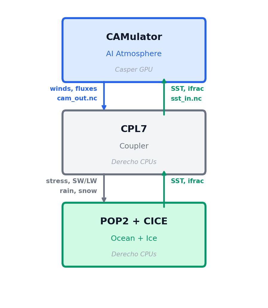
Instead of reading CORE2/JRA55 forcing files, DATM_MODE = CAMULATOR calls our Python inference server via the filesystem:
Every 6 hours:
  DATM writes  → sst_in.nc  (SST from POP2)
  DATM writes  → go.flag
  [polls every 1s, timeout 1h]
  DATM reads   ← cam_out.nc (10 flux fields)
  DATM reads   ← done.flag
Two files changed in CESM source:
- New:
datm_datamode_camulator.F90 - Wired into:
datm_comp_mod.F90(case('CAMULATOR'))
Activated by DATM_MODE = CAMULATOR in user_nl_datm
Why file-based interface?
- No Fortran↔︎Python interop (no FTORCH/FORPY, no sockets)
- 6-hr coupling interval → ~10 MB I/O overhead is negligible
- Fully debuggable: inspect every
sst_in.ncandcam_out.ncindependently - Model-agnostic: swap
camulator_server.pyfor any CREDIT model — Fortran side never changes
Key physics handled server-side:
- SST/IFRAC injected into forcing tensor
- FSNS → FSDS: albedo inversion so CPL7 doesn’t double-count surface reflection
- FLNS → FLDS: isolates downwelling component
- Over-land SST fill for continental grid points
- Dynamic boundary layer height (
z_bot ∝ T_bot)
Flux Conversions: Net → Downwelling
CAMulator outputs net fluxes at the surface. CPL7 expects downwelling fluxes and applies surface albedo internally — so we have to invert before handing off.
SW — albedo inversion
\[\text{FSDS} = \frac{\text{FSNS}}{1 - \alpha_\text{sfc}}\]
\[\alpha_\text{sfc} = (1-f_\text{ice})\times 0.06 + f_\text{ice}\times 0.60\]
Passing FSNS directly would double-count the reflection — CPL7 applies albedo again internally.
\(f_\text{ice}\) is taken from CICE at the same timestep so the correction always tracks actual ice cover.
LW — Stefan-Boltzmann reconstruction
\[\text{FLNSD} = 0.99\,\sigma T_S^4 + \frac{\text{FLNS}}{\Delta t}\]
CAMulator gives net upward LW (FLNS). Adding back the upward surface emission (\(0.99\,\sigma T_S^4\)) isolates the downwelling component that CPL7 needs to force the ocean.
Dynamic \(z_\text{bot}\) and Monin-Obukhov Theory (?)
CPL7’s COARE-style bulk scheme needs the reference height \(z_\text{bot}\): the height of the data read in to compute the M-O stability correction and from that the wind stress \(\tau\), sensible heat \(H\), and latent heat \(LE\).
In CAM6 it’s not a fixed number; it varies ~50–67 m with surface temperature. We derive it consistently from the hybrid coordinate and the hypsometric equation:
\[p_\text{mid} = \underbrace{a_{N-1} p_0}_{\approx\, 0} + \frac{b_{N-1}+1}{2}\, p_s \;\approx\; \frac{b_{N-1}+1}{2}\, p_s\]
\[z_\text{bot} = \frac{R_d}{g}\ln\!\frac{p_s}{p_\text{mid}} \cdot T_\text{bot} \approx \frac{R_d}{g}\left(-\ln\frac{b_{N-1}+1}{2}\right) T_\text{bot} \approx 0.219\, T_\text{bot}\]
Getting \(z_\text{bot}\) wrong changes which stability regime CPL7 thinks it’s in.
- In stable conditions (cold SST under warm air), a wrong \(z_\text{bot}\) artificially suppresses wind stress
- In unstable conditions (warm tropical SST), it sets the strength of the convective enhancement of \(H\) and \(LE\)
These aren’t small corrections and this is the thing I’m most neverous about
For example: the Southern Ocean, Arctic margins, the MJO warm pool, and eastern boundary upwelling zones all spend significant time in strongly stratified regimes.
Speed: How does 42 SYPD Compare?
| Configuration | Speed (SYPD) | Hardware |
|---|---|---|
| Full CESM2 (CAM6 + POP2) | ~7.3 | 8 Derecho nodes |
| GIAF (DATM + POP2, no AI) | 37.935 | 2 Derecho nodes |
| CAMulator + POP2 (this work) | 42.025 | 2 CPU + 1 A100 |
Note
we get a prognostic, interactive atmosphere at roughly the same wall-clock cost as prescribed forcing and 6X cheaper than running full CAM6 + POP2.
Per-step breakdown on A100 (ms):
| Stage | Time |
|---|---|
| Build input tensor | ~5 |
| CAMulator inference (JIT) | ~190 |
| Inverse transform | ~8 |
| Grid remap (T62 ↔︎ 1°) | ~3 |
| Write cam_out.nc | ~15 |
| Total server time | ~220 |
CAM6 reference: one 6-hr step ~4932 ms on 8 CPU Nodes
CESM’s ocean/ice compute is the wall-clock bottleneck — not inference.
Movie: Monthly SSTs and Precip
Movie: ENSO
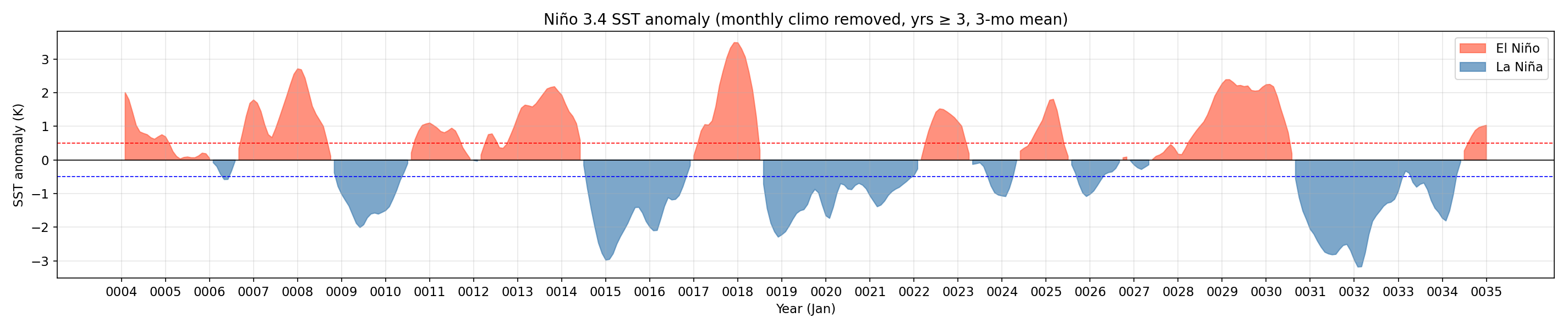
ENSO: Niño 3.4 Index
The coupled run produces realistic interannual SST variability in the tropical Pacific — ENSO cycles emerge spontaneously from the coupled system.
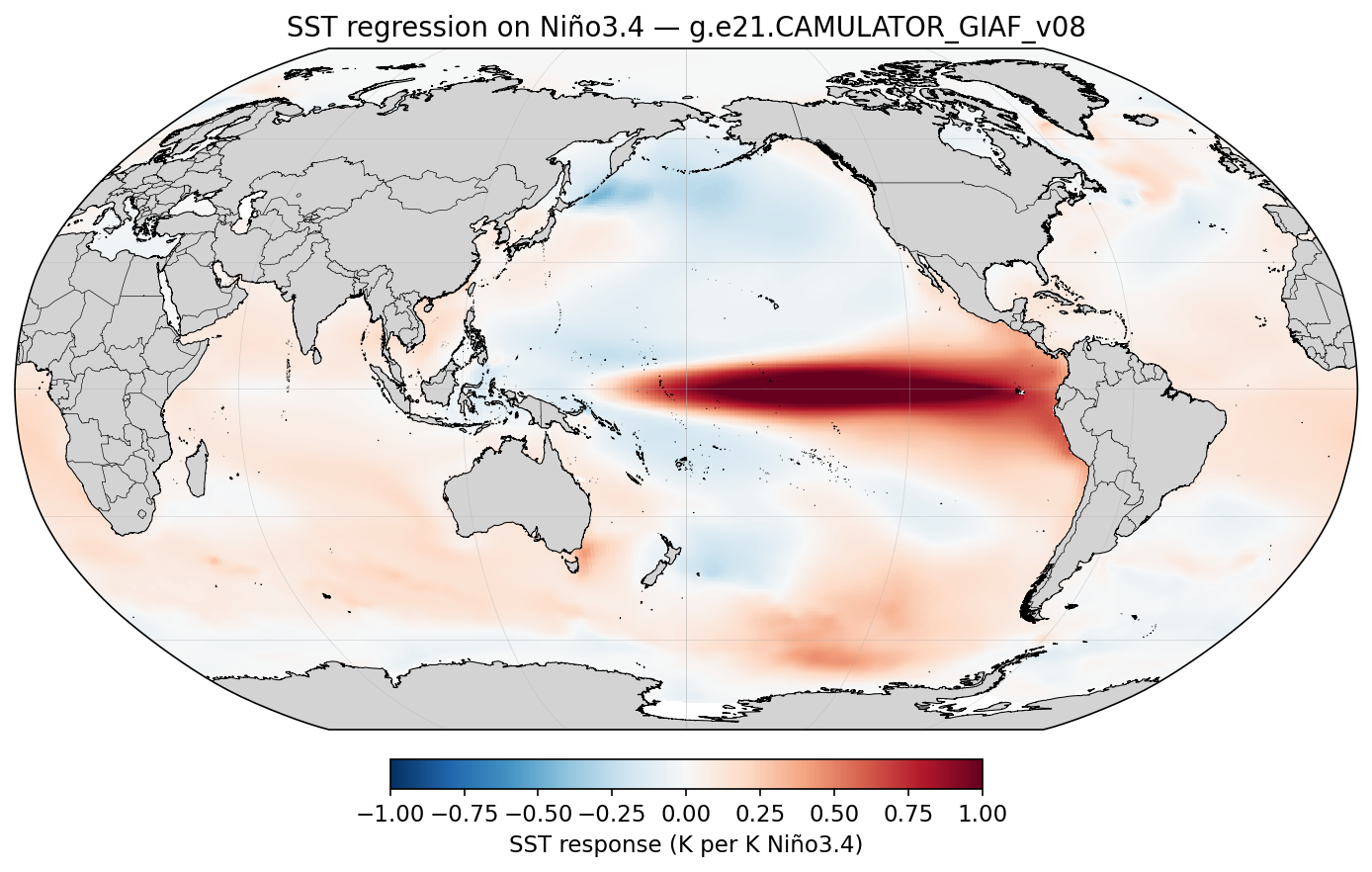
ENSO: Spatial Pattern
SST regression on Niño 3.4 shows the correct east-Pacific warming structure and horseshoe cooling in the off-equatorial Pacific.
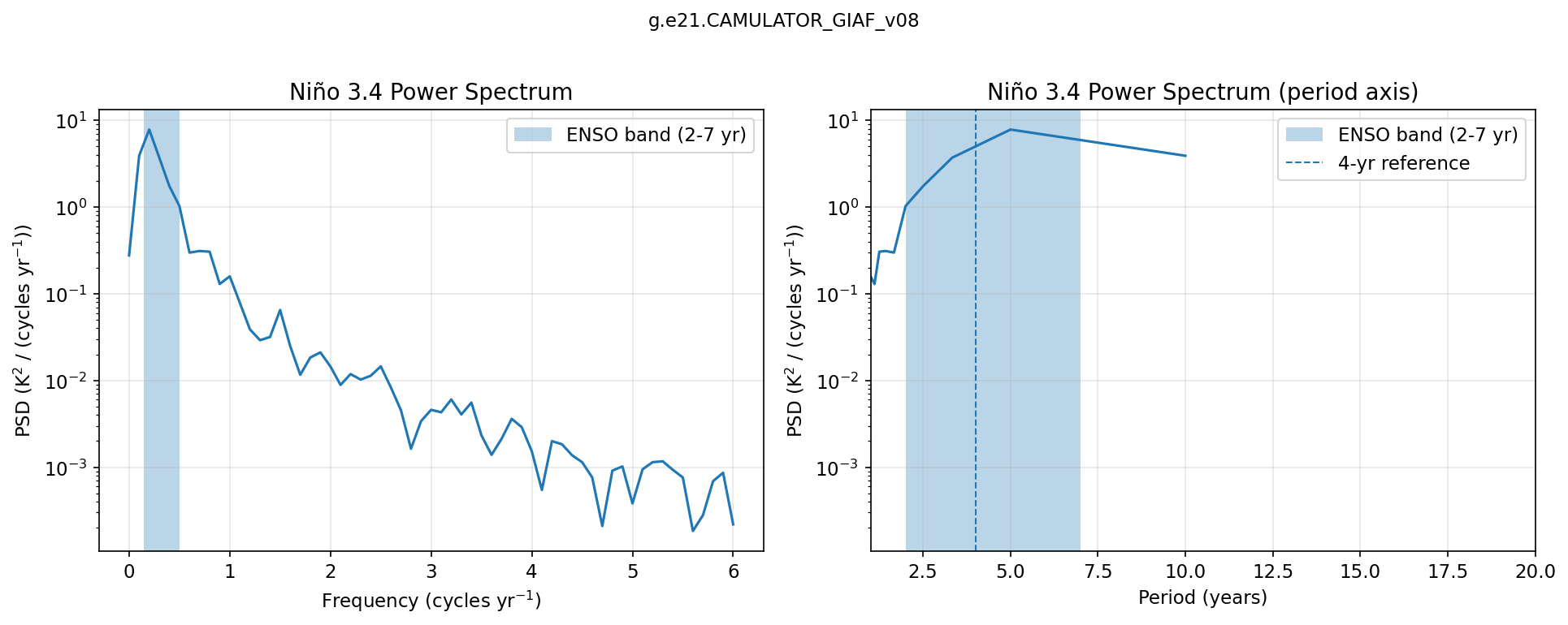
ENSO: Power Spectrum
Spectral power peaks within the 2–7 year ENSO band, consistent with observed ENSO periodicity.
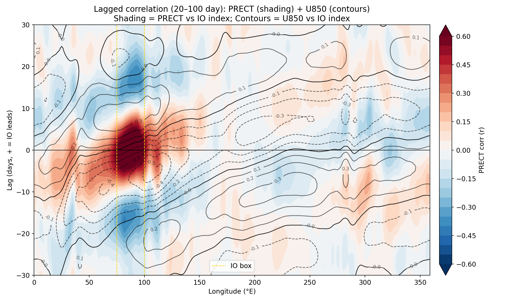
MJO: Lagged Correlation
The coupled run captures eastward-propagating convective anomalies on intraseasonal timescales — precipitation and 850 hPa wind both track the Indian Ocean signal with the correct-ish phase relationship.
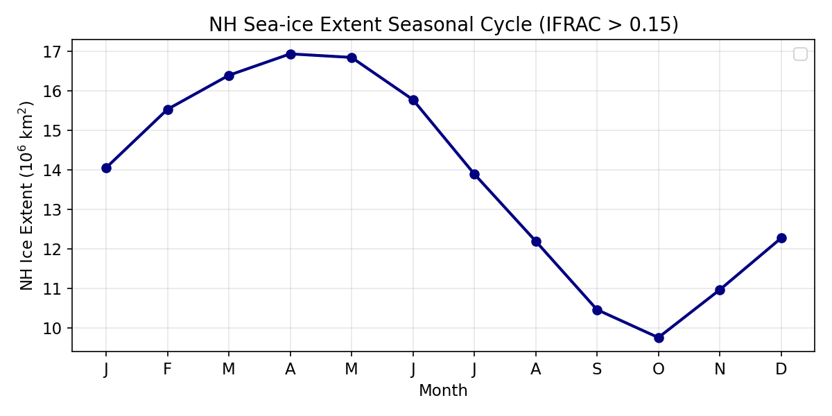
Results: Northern Hemisphere Sea Ice
NH sea ice extent follows a realistic seasonal cycle with no runaway loss or gain over the 35-year run.
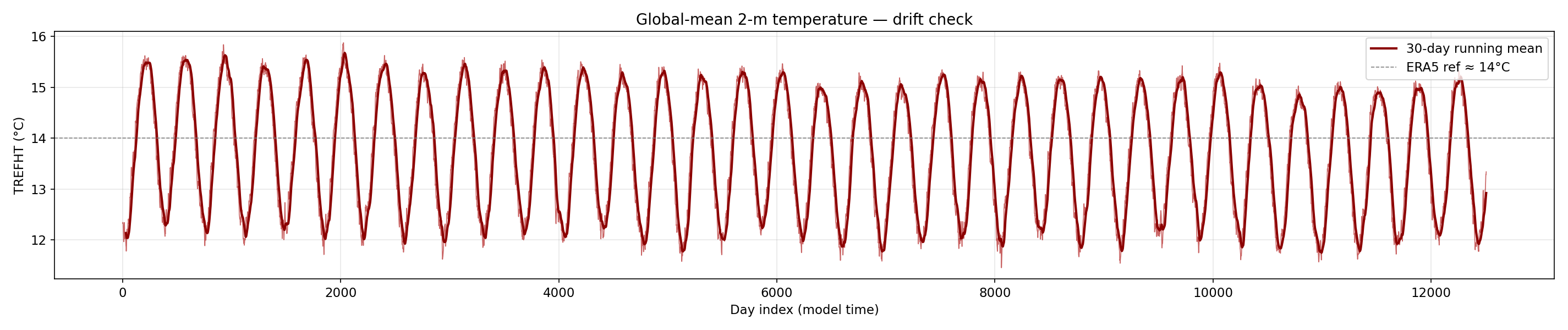
Results: Global Mean Temperature
Global-mean 2m air temperature shows no long-term drift over the 35-year run — the coupled system is stable (ish).
What 42 SYPD Enables
With a large speedup over CAM6, coupled experiments become feasible that weren’t before:
- Large ensembles with interactive ocean — 50–100 member ENSO forecasts at seasonal range
- Centennial runs to study climate drift, AMOC stability, heat uptake
- Parameter sensitivity sweeps — vary ocean mixing, ice albedo, test parameterization choices at low cost
- Rapid prototyping of new coupling strategies before investing in full CESM runs
The flag-file interface is intentionally model-agnostic:
The Fortran side (datm_datamode_camulator.F90) never changes. Any model that can read sst_in.nc and write cam_out.nc can be plugged in.
Next Steps
Science questions now open:
- ENSO response — does CAMulator + POP2 produce realistic ENSO amplitude and period? Does it improve over OMIP?
- Creating an ACE2 Sever is Trivial in CREDIT - what ocean biases emerge with a reanalysis atmosphere?
- MJO air-sea feedback — does the interactive atmosphere change MJO propagation speed or coherence?
- Creating an ACE2 Sever is Trivial in CREDIT - what ocean biases emerge with a reanalysis atmosphere?
- Creating an ACE2 Sever is Trivial in CREDIT - what ocean biases emerge with a reanalysis atmosphere?
- AMOC stability — multi-decadal runs with changing wind stress
- SST bias evolution — does CAMulator’s known high-latitude cold bias change ocean heat uptake?
- Ensemble spread — do coupled members diverge faster than AMIP/OMIP members? S2S simulations
- Ocean stuff, I know next to nothing about the ocean.
- Does calibrating ocean with this atmosphere help the bottleneck?
Technical next steps:
- Phase 2: bypass CPL7 bulk formula — pass
Faxa_taux/tauydirectly instead ofSa_u/Sa_vand Latent / Sensible Heat - Retrain CAMulator to directly simulated downward fluxes at surface
- MOM6 coupling (CESM3 ocean)
- Just switch the compset and this should(?) work now.
Community:
- CESM patch +
camulator_server.py→ open release - Generalise server interface for any CREDIT model
- Share restart-safe launch scripts with the community
Summary
We coupled an AI atmosphere to a dynamic ocean by:
Writing a new DATM datamode (
CAMULATOR) — zero coupler modifications, file-based flag I/O, fully debuggableTried to get the physics right: FSNS→FSDS albedo inversion so CPL7 doesn’t double-count surface reflection; dynamic \(z_\text{bot}\) derived from hybrid coordinates for physically consistent M-O stability corrections
Running it: 42 SYPD, 35-year run stable, POP2 + CICE receiving evolving AI-generated fluxes and feeding SST back at every step
(Also had to fix a deep CPL7 pointer bug where xao_ax was never assigned for DATA ATM — see Appendix)
42 SYPD + prognostic ocean = multi-century coupled experiments at a fraction of the cost of full CESM
Appendix
Slides below contain implementation detail for follow-up discussion
A: Component Glossary
| Component | Role in this project |
|---|---|
| CESM2/CPL7 | Framework + MCT-based Fortran coupler; remaps fields between grids, applies bulk formulae |
| DATM (Data ATM) | Normally reads CORE2/JRA55 prescribed forcing. Here: runs CAMULATOR mode — a new datamode we wrote |
| CAMulator | Autoregressive 6-hr AI atmosphere trained on CAM6 output. 192×288 (1°), 130 prognostic channels |
| POP2 | 3D ocean on gx1v7 displaced-pole grid (~1°, 320×384). Evolves SST, salinity, currents |
| CICE | Sea ice on same gx1v7 grid. Exchanges heat, momentum, freshwater with POP + atmosphere |
| T62 grid | DATM’s native Gaussian grid: 94 lat × 192 lon. All DATM→CPL fields live here |
| GIAF compset | DATM%IAF + POP2 + CICE — the baseline we piggyback on |
B: Full Architecture
┌─────────────────────────────────────────────────────────────────────────┐
│   CESM2 CPL7 coupled run   (Fortran/MPI, CPU ranks on Derecho)          │
│                                                                          │
│   POP2 ──SST──► CPL7 ──x2a_So_t──► DATM (CAMULATOR mode)               │
│                                          │                               │
│                              write camulator_sst_in.nc                   │
│                              write camulator_go.flag   ───► [GPU server] │
│                                          ↑                               │
│                              read  camulator_done.flag ◄─── [GPU server] │
│                              read  camulator_cam_out.nc                  │
│                                          │                               │
│   POP2 ◄──a2x fluxes──── CPL7 ◄──────────┘                              │
└─────────────────────────────────────────────────────────────────────────┘
                   ▲ shared GLADE filesystem
┌──────────────────┴──────────────────────────────────────────────────────┐
│   camulator_server.py  (Python, A100 GPU, pre-launched on Casper)        │
│                                                                          │
│   loop:  watch go.flag → read sst_in.nc → inject SST → run CAMulator    │
│          → write cam_out.nc → write done.flag                            │
└─────────────────────────────────────────────────────────────────────────┘
C: Grid Remapping
| Grid | Dims | Used by |
|---|---|---|
| T62 Gaussian | 94 × 192 | DATM, CPL7 |
| CAMulator 1° | 192 × 288 | AI model |
Precomputed BilinearRemap weights at startup → remap ~2.5 ms (vs ~500 ms with RegularGridInterpolator every step)
T62 Gaussian latitudes computed exactly:
class BilinearRemap:
    """Precomputed bilinear weights for T62 ↔ CAMulator."""
    def __init__(self, src_lat, src_lon,
                       dst_lat, dst_lon):
        # compute weight matrices once at startup
        ...

    def batch(self, fields_dict: dict) -> dict:
        """Remap all fields in one vectorised call."""
        out = {}
        for name, arr in fields_dict.items():
            out[name] = (self.weights @ arr.ravel()
                         ).reshape(self.dst_shape)
        return out
D: SST Injection Detail
# 1. Read SST from sst_in.nc [K]
sst_t62 = ds['sst'].values           # 94×192

# 2. Remap T62 → CAMulator 1° grid
sst_cam = remap_t62_to_cam(sst_t62)  # 192×288

# 3. Over-land fill (POP only provides ocean points)
mask = sst_cam > 270.0               # True = ocean
sst_blended = np.where(mask, sst_from_pop, 283.0)

# 4. Normalize and inject into forcing tensor
sst_norm = (sst_blended - sst_mean) / sst_std
model_input = stepper.state_manager \
    .build_input_with_forcing(state, forcing_t, static)
accessor_input.set_state_var(model_input, 'SST', sst_norm_tensor)

# 5. Run inference
prediction = stepper.model(model_input.float())
SST is a dynamic_forcing_variable (not prognostic state) — it lives in the forcing tensor, not in the 130-channel prognostic state. This is why injection works without retraining the model.
E: Flux Conventions
| Variable | CAMulator units | → cam_out.nc |
|---|---|---|
FSNS |
J m⁻² (6h total) | ÷ 21600 → W m⁻² |
FLNS |
J m⁻² upward | ÷ (−21600) → W m⁻² ↓ |
PRECT |
m s⁻¹ liq-eq | direct |
TAUX/TAUY |
Pa | direct |
SW albedo inversion: \[\text{FSDS} = \frac{\text{FSNS}}{1 - \alpha_\text{sfc}}\] \[\alpha_\text{sfc} = (1-f_\text{ice}) \times 0.06 + f_\text{ice} \times 0.60\]
CPL7 treats Faxa_sw* as downwelling and applies albedo internally — passing FSNS directly double-counts it.
F: Restart Handling
ATM restart file (camulator_atm_restart.pth):
On CONTINUE_RUN=TRUE, CESM re-sends the last go.flag. Server detects current_ymd == last_ymd, re-sends saved cam_out without re-inference.
G: Launch Workflow
sequenceDiagram
    participant U as User (login node)
    participant S as camulator_server.py (Casper A100)
    participant C as CESM (Derecho CPU nodes)
    participant G as GLADE filesystem

    U->>S: qsub server job (Casper)
    S->>S: load model, JIT trace (~60s)
    S->>G: write camulator_server_ready.flag

    U->>U: launch_coupled_run.sh polling...
    U->>C: case.submit (triggered by ready flag)

    loop Every 6 hours
        C->>G: write sst_in.nc + go.flag
        G->>S: server detects go.flag
        S->>S: inject SST, run inference (~200ms)
        S->>G: write cam_out.nc + done.flag
        G->>C: DATM reads cam_out.nc
        C->>C: CPL7 remaps, applies bulk formula
        C->>C: POP2 + CICE advance one step
    end

    C->>G: write restart files (annual)
    S->>G: write camulator_atm_restart.pth
H: The CPL7 Bug
Symptom: Ocean sees SST = 0 K on every coupling step despite POP sending valid temperatures.
Root cause — cime_comp_mod.F90:
The xao_ax pointer (ATM↔︎OCN flux object) is initialised only inside:
For DATA ATM (atm_prognostic = .false.), this block is never entered → xao_ax stays null().
Later at every coupling step:
No one had ever run a DATA ATM that needed to read back ocean state — this code path had never been exercised in 20 years of CESM.
Three-part fix (all in ATM SETUP-SEND block):
Fix 1 & 2 — widen two guards from atm_prognostic to (atm_prognostic .or. atm_present):
Fix 3 — assign pointer before the associated() check:
Confirmed: 10-day coupled run at 42 SYPD ✅
CAMulator ↔︎ POP2 Coupling | CU Boulder/M2LINES